
PFM Class
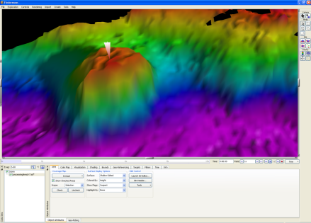
All PFM viewing and manipulation is done through the main Fledermaus interface. The following section describes the capabilities of viewing and editing PFM files within Fledermaus.
The data in the PFM bins are used to build regularly gridded surfaces that describe the shape of the terrain and can be explored using normal exploration methods. The individual records and their attributes can also be displayed for selected regions in the 3D Editor. Some features of the PFM object's data controls are:
- Switch between six DTM's: filtered and unfiltered surfaces of shallowest, average and deepest sounding in each bin.
- Color-code the DTM by depth, standard deviation, sounding density, various flags, or by attribute.
- Highlight suspect, plotted, or feature soundings in the data set.
- Display the DTM semi-transparent or as wire frame.
- Select and view soundings and their attributes in the 3D editor.
- Create and export the DTM to a separate SonarDTM object at any time.
- Tools to export and apply exported edits on the PFM.
When a PFM data object is selected in the data set control you will be presented with the controls shown in Figure 137.
Coverage Control Panel
Once a PFM file has been loaded as described in Figure 137, the Coverage Control Panel will be shown by default when the object is selected from the Data Set Control. Bins that contain data that have been checked will appear light grey and those not checked will be red.
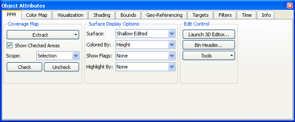
Figure 1 37 - Coverage Control Panel
A surface object is created for visualization by highlighting a region on the coverage map by holding down the left mouse button and dragging the mouse until the desired region is enclosed in the selection rectangle. After selecting the area press the right mouse button and select Extract Selected Region. To load the whole surface from the PFM press down the right mouse button and select Extract Entire Area (see Figure 138). The dimensions of the selected area (in meters) are shown in the Area text field. 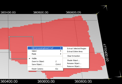
Figure 1 38 - Extraction of PFM Data for Visualization
In addition, the PFM Coverage Control panel has specific tools for working with the surface. The first option is the Surface pull-down menu, which provides a choice between displaying the unfiltered shallow, average or deep surfaces, along with the filtered shallow, average or deep surfaces. The unfiltered surface shows a surface from all available soundings in the PFM file while the filtered surface does not include soundings marked as deleted. The Color pull-down menu directly below the Surface selection menu provides a choice of the attribute used to color the surface:
- Standard deviation;
- Height;
- Sounding density;
- Deleted flag;
- Modified flag;
- Checked flag;
- Suspect flag;
- Plotted flag;
- Feature flag;
- File number;
- Line number; and,
- Custom Flags or Attributes (if they exist).
The Highlight menu allows areas of the PFM that have a certain flag set to be highlighted in the main display (highlighted areas will appear lighter than the surrounding areas). Select one of the available flags from the Highlight menu to enable this option. Using highlighting, it is possible to visualize more than one variable at a time (e.g. the surface could be colored by depth and the areas that are checked could be highlighted).
There is also an option to directly display what bins contain either selected, plotted, or feature soundings. This can be controlled using the Flags pull down. When either of the flags is selected, markers will appear on the surface indicating which bins contain soundings with the given flag (see Figure 139). This option is independent from the set color of the surface. The setting of the flags will be from either the functions on the Filters Panel or from manual edits in the 3D Editor.
As the processing continues, the Check button allows the users to set areas that have already been processed and approved. This can then be shown on the visualized surface and also in the overview on the Coverage Control panel, as shown in Figure 137. The checked areas will be displayed as grey on the Coverage Map when the Show Checked Areas toggle is enabled. The Check button sets all bins in an area as checked and the Uncheck button undoes this process. The area that is set or reset depends upon the value of the Scope drop-down list. When the scope is Loaded Area, the extracted area is modified; when the scope is Selection, only the area chosen using the Select Mode is modified; when the scope is Entire PFM File, the whole file is modified. Setting or resetting checked areas is recorded in the Audit file.
The remaining controls on the Coverage Control panel are related to the analysis and editing of the underlying sounding data. Some of these options require a selection on the surface that can be accomplished by entering the Select mode on the top right of the application and clicking and dragging on the surface. The available options in the Edit Control box are outlined as follows:
Launch 3D Editor – runs the Fledermaus 3D Editor on the selected area. Also can be started by pressing the '3' key. See Section 3D Editor for a full description.
Bin Header -- Displays summary information about the PFM file, as shown in Figure 140.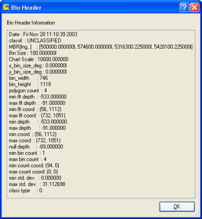
Figure 140 - Bin Header Dialog Box
The Tools menu button has the following options:
Launch Area Editor – runs the NAVO editor tool on the selected area. This option only works under Linux and the PFM_EDIT environment variable must point to the editor path.
Create Surface Object – creates a SonarDTM of the currently extracted area. The new surface will appear in the Data Set Control list.
Export Soundings – writes all soundings in a specific area to a variety of formats including ASCII XYZ, ASCII XYZ + Attributes, and NAVO/Caris ascii files. The area to extract can be chosen using the Export Soundings dialog as shown in Figure 141. Choose the Selection toggle to output all soundings in the selection box on the surface, choose Loaded Area to output all soundings in the extracted area, or export all soundings in the file by choosing the Entire PFM File toggle. The set of soundings to export can be chosen using a combination of the Base Sounding Selection On area, and the Refine Selection Based On Sounding Flags area. Use the Base Soundings Selection On area to choose whether just accepted soundings, rejected soundings, or both are output to the file. If any of the checkboxes in the Refine Selection Based On Sounding Flags area are turned on, then only the soundings that have one of those flags set are output to the file. Turning on the Automatically Unproject Soundings if Necessary toggle when the data is in the UTM projection causes the soundings to be converted to geographic coordinates before exporting. The data can be output as ASCII XYZ by selecting Ascii XYZ Only from the Select Output Format drop-down list. Selecting Ascii XYZ + Attributes exports any available PFM attributes as well as the x, y, and z locations, and finally the soundings can be exported in a special ASCII format used by NAVO and Caris by selecting NAVO/CarisAscii from the list.
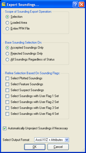
Figure 141 - Export Soundings Dialog
Export Shoal Soundings – outputs a text file that contains a set of XYZ points representing the shoalest sounding in each bin of the selected area (see Figure 142). The selected area can either be Selection (use the select tool to highlight an area), Loaded Area (the entire area that has been extracted), or Entire PFM File (the whole file). If the Automatically Unproject Soundings if Necessary toggle is set and the data is in UTM projection, the soundings will be converted to geographic coordinates before they are output. The output format can be specified with the Select Output Format drop-down list and can either be Ascii XYZ Only, Ascii XYZ + Attributes, or NAVO/CarisAscii.

Figure 142 - Export Shoal Soundings Dialog
Export Survey Lines – this option writes a list of all survey lines that intersect the indicated area to an ASCII file. The area to check can either be Selection to output lines just in the selection box, Loaded Area to output lines in the extracted area, or Entire PFM File to output all lines in the PFM file.
Export Survey Files – this option writes a list of all survey data files that intersect the indicated area to an ASCII file. The area can either be set to the selection box by choosing the Selection toggle, the extracted area by selecting the Loaded Area toggle, or the entire PFM by selecting the Entire PFM File toggle.
Bin Info - displays a dialog box, shown in Figure 143, with a number of fields that contain information in each bin. Once the dialog box is shown, move the cursor over the surface in the Explore mode and the fields will display the data for the bin closest to the cursor position.
Cube – contains a submenu with a number of options for working the Cube PFMs. See CUBE Tools for more information.
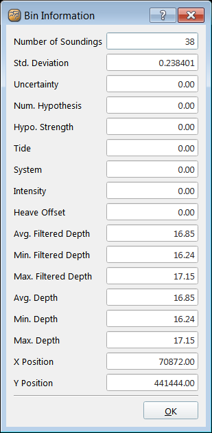
Figure 143 - Bin Info Dialog Box
Visualization Control Panel
The Visualization Control panel is used to adjust the display options for the extracted PFM bin file. The extracted surface can be manipulated with many of the same Fledermaus tools available for SonarDTMs. These include geo-picking coordinates, profiling, contouring, and re-shading.
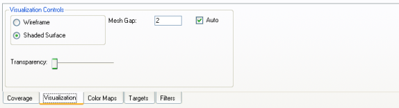
Figure 1 44 - Visualization Control Panel
The Transparency, Mesh Gap, Auto, Wireframe, and Shaded Surface controls are used to control the appearance of the DTM. These controls are similar to those for a regular SonarDTM (see Chapter 3 in the Fledermaus Reference Manual).
Targets Panel
A target, sometimes called a contact, is a special point of interest with a number of attached attributes and possibly an attached snippet image file. Targets are stored in a separate XML file using the standard NAVO target format and the file name of the XML file is stored within the PFM file. When a PFM file is loaded containing a valid targets file, the targets will automatically be displayed and can be editing using the Targets panel shown in Figure 145. Note that targets have only a latitude and longitude position and no depth value is stored (targets are usually displayed as lying on a surface if one is available at the location of the target).
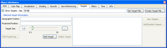
Figure 1 45 - Targets Panel
Targets are displayed as spheres in a scene and can be hidden or shown using the Show Targets toggle. The current target file is displayed in the text field at the top of the panel. If a target file exists but is not associated with the current PFM, click the Set Target File button and select the XML file using the standard file dialog box. To create a new targets file, click the Create Target File button and select a new file to create.
If multiple targets exist in the scene the targets will be displayed as yellow. To select a target, enter Select mode and then click near a target. The target will change color to white, indicating that the target is selected and information about the target will be displayed in the Geographic and Projection Position fields. As well, information from the XML file will be displayed in the text area to the right of the fields. To move the target to a new position, click the Edit Positioning button and enter the geographic position of the target in the dialog that is displayed.
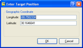
Figure 1 46 - Adding or Moving a Target
To add a target, click the Add Target button and enter the geographic position of the target in the dialog that is displayed (see Figure 146). Note that if a point is picked on the surface of a DTM while in Select mode (a white cross will appear on the surface), then the position of the last picked point will be displayed in the Enter Target Position dialog. To delete a target, click on the target while in Select mode and click the Delete Target button.
Some targets have an associated snippet image. If a snippet exists for the target, click the View Snippet button and the image will be loaded in displayed in a separate dialog (see Figure 147). To associate a snippet image with a target, select the target, click the Add/Update Snippet button, and select a valid image file.
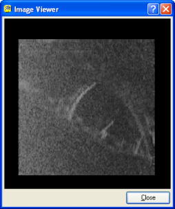
Figure 1 47 - Viewing a Snippet Associated with a Target
Targets can also be added, deleted, and moved using the 3D Editor.
Filters Panel
The Filters Panel allows filters to be run on the current PFM file and is shown in Figure 148. All operations in this panel depend on the setting of the Scope pull down menu. The different options for the scope are as follows:
- Selection – area selected by dragging with the mouse in Select mode;
- Loaded Area (default) – currently extracted area; or,
- Entire PFM File – all soundings in the PFM file.
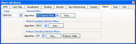
Figure 148 - Filters Panel
Three types of operations exist in the Filters panel: Select, Clear, and Export. Each operation can be run on the Suspect, Plotted, or Feature flags and the buttons for each flag are located to the right of the flag label. The Select button will run a filter on all soundings in the selection scope to automatically set flags of a certain type. The Clear button will remove the given flag from all soundings in the given selection scope. To save all soundings in the selection scope that have a certain flag, click the Export button.
Selecting Suspect Soundings
The suspect soundings selection filter assists the user in identifying soundings that may be incorrect. Clicking the Select button beside the Suspect Soundings label will display the Suspect Filter Options dialog, shown in Figure 149. The filter will select all soundings with depths that are more than a certain threshold away from the average depth in a bin. Enter a threshold in the Depth Threshold Difference text field and click the Filter button.
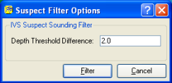
Figure 1 49 - Filter Options for Suspect Soundings
Bins that contain suspect soundings can be shown by setting the Color popup menu to Suspect or the Flags menu to Suspect on the Surface Control panel.
Selecting Plotted Soundings
Automatically selecting soundings for plotting can be accomplished through the Select button to the right of the Plotted Soundings label. This operation is used to run a sounding selection algorithm and will display the dialog box as shown in Figure 150. Normally the chart scale is specified to determine the default distance between selected soundings that are entered in the Chart Scale text field. For example a value of 20000 implies a chart scale of 1:20000. This gives the default minimum distance between soundings and is based on assuming 5mm text for the resulting chart. You can directly enter the minimum distance, overriding the suggested default for the given chart scale, by typing a new value in the Minimum Distance text field. The Selection Factor that defaults to four is used in algorithm and generally should be left alone. A smaller number improves the quality of the selection but increases running time (the default has been found to be a good balance). The Parameter Status field shows the criterion for running the algorithm. You cannot select soundings if you select an unreasonable chart scale for the bin size of the PFM. The dialog box will display a message just below the parameter status to indicate if the selected parameters are acceptable or not. If they are not you must increase the chart scale (or minimum distance).
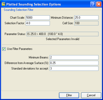
Figure 1 50 - Filter Options for the Plotted Soundings Algorithm
If advanced filters are to be used with the selection algorithm, enable the Use Filter Parameters toggle. Before being selected by the filter, the sounding must pass three criteria: it must be in a bin with more than a certain number of soundings, its height must be far enough away from the average bin height, and the standard deviation of the sounding must be above a certain level. Enter values in the Minimum Beams, Difference from Average Surface (0.25 = 25%), and Standard Deviations for accept text fields respectively to control these options. If Use Filter Parameters is off, the bottom three text fields are ignored. Click the Filter button to run the filter on the selection scope.
Setting the Color popup menu to Plotted or the Flags menu to Plotted on the Surface Control panel will display which bins contain the plotted flag.
Selecting Feature Soundings
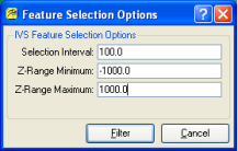
Figure 1 51 - Filter Options for Feature Soundings
Selecting feature soundings is performed by clicking the Select button to the right of the Feature Soundings label. This will display the dialog as shown in Figure 151. Specify the minimum distance apart of shoals in the horizontal plane (Selection Interval), and specify the depth range for consideration in the Z Range Minimum and Z Range Maximum text fields. Click the Filter button to begin the algorithm.
The actual algorithm is a two-step process. In the first step, the process searches through all the data based on the defined cell size and finds the shallowest sounding that is not flagged as deleted and is within the selected depth range. In addition, the entry of the minimum and maximum values allows the user to restrict the process to only those soundings within the selected depth range. The second step prunes the list of selected shoal soundings based on the range interval entered. In this step, the selected soundings are first sorted in descending order. The shallowest is selected and then any sounding that lies within the entered range is deleted. The next shallowest sounding is selected and any soundings that lie within the entered range to it are deleted.
Soundings with the feature flag set can be shown by setting the Color popup menu to Feature; or the Flags menu to Feature on the Surface Control panel. Also, a list of feature soundings can be shown by clicking the Table button to the right of the Feature Soundings label.
Feature Soundings Table
The Feature Soundings Table is used for both the displaying and working with the data records that have been flagged as features. The selected sounding in the table will be highlighted and will also be highlighted by a red stalk in the Fledermaus window. If further details of the data point are required, the details can be examined in the same manner to the 3D Editor table (Error! Reference source not found.). On completion the table can be saved as an ASCII file for use elsewhere by right clicking on the table and selecting Save PFM Table As.
Export and Apply Edits
In the Tools dropdown, there are two entries to export and apply exported edits on the PFM. This permits a combination of saving specific types of edits, which are: manually rejected, filter rejected, suspect, plotted and feature flagged edits. This way, specific edits can be applied to a fresh, unedited copy to see the effect, remove unwanted edits or migrate the edits to a new version of PFM. Click on Export PFM Edits to select the flags to save. The edits must be saved to an empty directory, which should be specified in the Name for Edits field. It is not possible save edits over existing edits. To apply the edits, click Apply PFM Edits and specify the name of the directory where the edits were saved.
Return to: Reference Manual