
Description
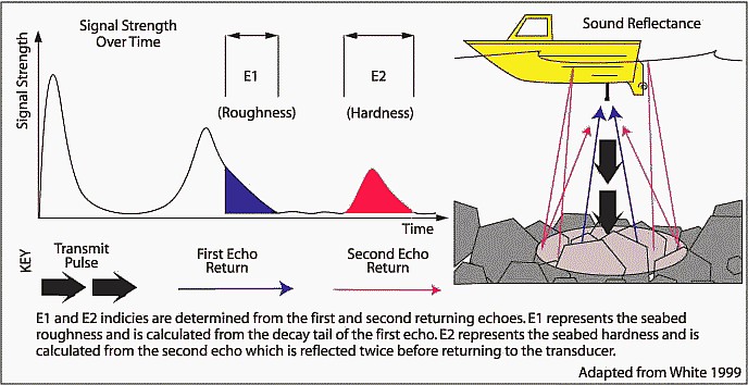
The RoxAnn system from company Sonavision can be used as a normal echosounder, but is also a so-called Acoustic Ground Discriminating System (AGDS).
It is capable of determining variability in the seabed type by combining data on the first (e1) and second (e2) echo pulses received by the same echosounder transducer.
Driver Information
|
Driver |
Sonavision RoxAnn (Bottom Classification) |
Interface Type |
Serial |
Driver Class Type |
Terminated |
|---|---|---|---|---|---|
|
No |
Input / Output |
Input |
Executable |
DrvQpsTerminatedUI.exe |
|
|
Related Systems |
|||||
|
Related Pages |
|
||||
Decoding Notes
Driver will automatically detect whether the Standard or the Deep Water data message is used.
Because the depth data field does not contain a real depth value, but a clock cycle counter, it is important to tell the driver the sound velocity and the frequency being used.
This is the responsibility of the user and should be done prior to the start of your survey and when settings have changed on the RoxAnn system itself.
The used sound velocity and the used frequency should be changed while online (see tab page Qinsy Online).
No time information is part of the message, therefore time stamping of the data is done when it arrives at the I/O port.
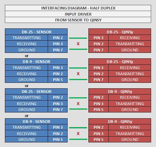
Interfacing Notes
The driver does not send any data or commands to the RoxAnn system, so only half-duplex wiring is needed:
Database Setup
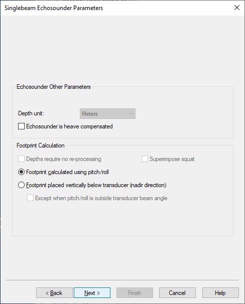
Add to your template setup a Singlebeam Echosounder system and select driver "Sonavision RoxAnn (Bottom Classification)".
Fill in the correct I/O parameters and press Next to go to the next wizard page.
Add three Transducers, each one with its unique Slot Id.
The selected node for each transducer should be the actual transducer location, and therefore the same for all three.
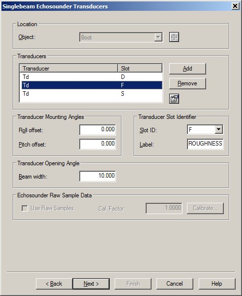
The decoded depth will be the same for all three transducers; the decoded intensity depends on the selected Slot Id:
|
Td |
Slot ID |
Label |
Observation Value |
Observation Intensity/Quality |
|---|---|---|---|---|
|
Td |
D |
BC |
Decoded Depth |
Bottom classification, calculated from E1 and E2 |
|
Td |
F |
ROUGHNESS |
Decoded Depth |
Decoded E1 (first echo return) |
|
Td |
S |
HARDNESS |
Decoded Depth |
Decoded E2 (second echo return) |
The label is free text to enter, it is recommended to use the labels from the table above.
In the online setup you can improve the reported depth with a better sound velocity than the one that will be used by default, in order to convert the decoded clock cycles from the D field into a depth value..
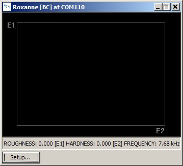
Online
The driver has user-interface, and therefore will always be present in the Windows taskbar.
When going on-line for the first time, locate the driver and change the Setup parameters.
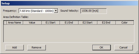
Frequency and Sound Velocity
The selected frequency, together with the sound velocity, will be used by the driver to convert the decoded clock cycles into a one-way depth.
The following formula is used: Depth = (Clock Cycles * Sound Velocity) / (2 * Frequency)
The used sound velocity can not be modified here. In order to improve the depth you need to change the Sound velocity mode in the Controller's Echosounder Refraction setup:
Controller
The Sound velocity mode can be found in the Controller's Echosounder Settings:
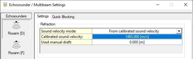
Here you should overrule the default sound velocity as used by the echosounder unit in order to improve the measured depth with a better sound velocity.
Select for Sound velocity mode: From calibrated sound velocity and then enter for the Calibrated sound velocity the same sound velocity that is used on the unit. It will be this sound velocity that you'll see in the driver's Setup dialog
-
As used by the unit (default but not recommended)
Qinsy will use the decoded depth value as reported by the unit.
Use this mode when you're confident that the used sound velocity is accurate enough for your survey specifications. -
From calibrated sound velocity
Use this mode when the echosounder unit is using a default/wrong/out-dated sound velocity and from your own measurement/calibration you have determined a better sound velocity value. -
From velocity profile (recommended)
Use this mode when your setup has an up-to-date sound velocity profile for your survey area.
This mode is recommended because ray-tracing will be used for the entire water-column instead of one fixed sound velocity value. -
From velocity observation
Use this mode when the echosounder unit is using a default/wrong/out-dated sound velocity and you have a sensor defined in your setup that measures in real-time an accurate sound velocity value.
Area Definition Table
The Bottom Classification value (BC) will be derived from the two decoded E1 and E2 values, therefore the user should create an Area Definition Table.
Note that the BC remains zero when the Area Definition Table is still empty.
Just use the Add button to add a new area, and set the boundaries for the E1 and E2 range.
Name the new area, e.g. "Sand" and assign a value representing the bottom classification code for this area type.
The selected color is only for displaying the area box in the main dialog of this driver.
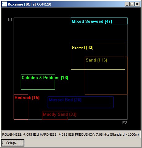
For example, the following areas have been added:
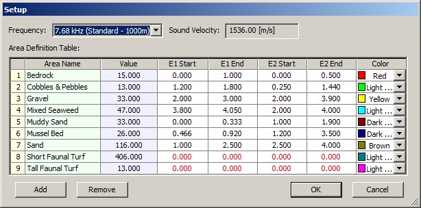
and in the driver this will look as follows:
Tip 
The setup of an Area Definition Table can be exported to a so-called xml file.
This file can be quickly imported into another setup which may be useful when having a vessel fleet operating in the same area: all vessels will then use the same definitions without having to enter all the individual values for each setup.
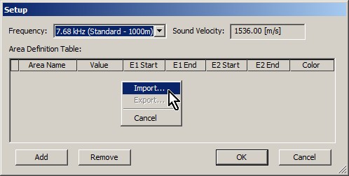
How? Just open the Setup dialog and use right-mouse popup menu to export or import the values.
Note that the user will be warned when importing new values from an xml file that the current definitions will be overwritten.
Display
The decoded data can be displayed using an Observation Physics Display or a Generic Display:
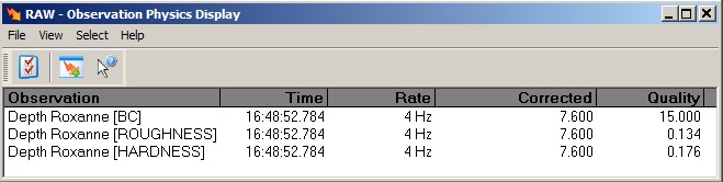
The decoded depth for all three transducers will be the same, so in the example above of the Observation Physics Display it is 7.6 meters.
The Quality indicator is used to display the calculated BC value (from the Area Definition Table) and the decoded E1 and E2 values.
So in the example above you see that: BC = 15, E1 = 0.134 Volts and E2 = 0.176 Volts.
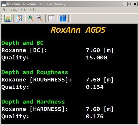
You may also use a Generic Display to show the same values as can be seen using an Observation Physics Display, however with this display you are more flexible to use your own layout, font size and color.
Sounding Grid
The decoded depth, the calculated BC and the decoded E1 and E2 values can each be stored in a separate sounding grid layer in order to show them as a geo-referenced color coded map:
Open the Session Setup, Storage, Sounding grid and select New...
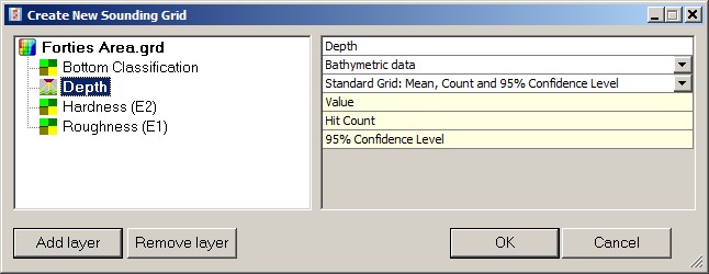
You may rename the default created layer 'Survey Data' into 'Depth' and you may also remove the Reference layer.
Subsequently add three new layers, and change for each layer the 'Bathymetric data' into 'Other data types'.
Change also the Standard Grid property into 'Simple Grid: Mean and Count'.
Rename the first new layer to 'Bottom Classification', the second one to 'Roughness (E1)' and the third one to 'Hardness (E2)'.
Select OK.
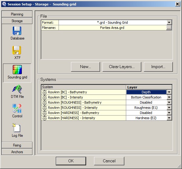
Intensity from the '[BC]' system should be stored in the newly created 'Bottom Classification' layer.
Intensity from the '[ROUGHNESS]' system should be stored in the newly created 'Roughness (E1)' layer.
Intensity from the '[HARDNESS]' system should be stored in the newly created 'Hardness (E2)' layer.
Bathymetry (i.e. the depth values) from only one of the systems should be stored in the newly created 'Depth' layer, so leave the layer for the other two Bathymetry systems Disabled.
The geo-referenced color coded map can be made visible online using a Navigation Display by selecting the required sounding grid layer, or offline using the Survey Manager.
Note that DTM File format QPD will also contain the intensity value for each enabled system.