How-to Computation Setup
This document describes how the Computation works in QINSy.
On this page:
Introduction
Least-Squares Network Adjustment
A least-squares adjustment is a mathematical procedure based on the theory of probability that derives the statistically most likely coordinate location of points/nodes defined by multiple measurements in a network. QINSy uses a full 3D model for the least-squares network adjustment which we call a 'computation'. All fixed and variable nodes, observations and offsets, together with their a-priori SD’s, are combined in a 3D network. This consists of a mathematical model that describes the relation of the unknown coordinates to the observations, and a stochastic model that describes the relative weights of the observations. All observations and their a-priori standard deviations (SD’s) enter the 3D adjustment directly without reducing or converting them. A least-squares adjustment is performed, in which all (valid) observations are adjusted so that the sum of the squares of the weighted observation residuals is minimized. If there is no redundancy of observations (no degrees of freedom), then there is nothing to adjust and no statistical testing can be done.
As designed in QINSy a least-squares adjustment (LSA) may go through the following three steps to find the best solution for a 3D network. If one step is unsuccessful, the next step is carried out:
- All observations, nodes and objects are added to the network. The LSA fails if the computation does not solve, does not iterate below its limit, or fails the F-Test. The computation will not solve if, for example, a USBL observation to an ROV is not available or is rejected, if multiple USBL observations do not iterate to a solution, or if one or more a-priori SD’s are too optimistic (SD value too low).
- Remove inter-object observations that have 'at nodes' on objects without absolute positioning. The LSA will try to compute a solution for a vessel and an ROV, if the vessel has an absolute positioning system and the ROV is positioned by USBL from the vessel, but not for a fish that is positioned by a manual layback from another fish that is positioned by manual layback or USBL. If the LSA is successful, the solution will be returned.
- Remove all inter-object observations from the network. All objects are computed independently using absolute positioning observations only. The LSA will not find solutions for objects without some absolute positioning system. The LSA will compute a solution for the vessel, but not for the ROV.
Note: 'Computation' and 'Adjustment' are used interchangeably in the text below.
Relative Weights of Observations
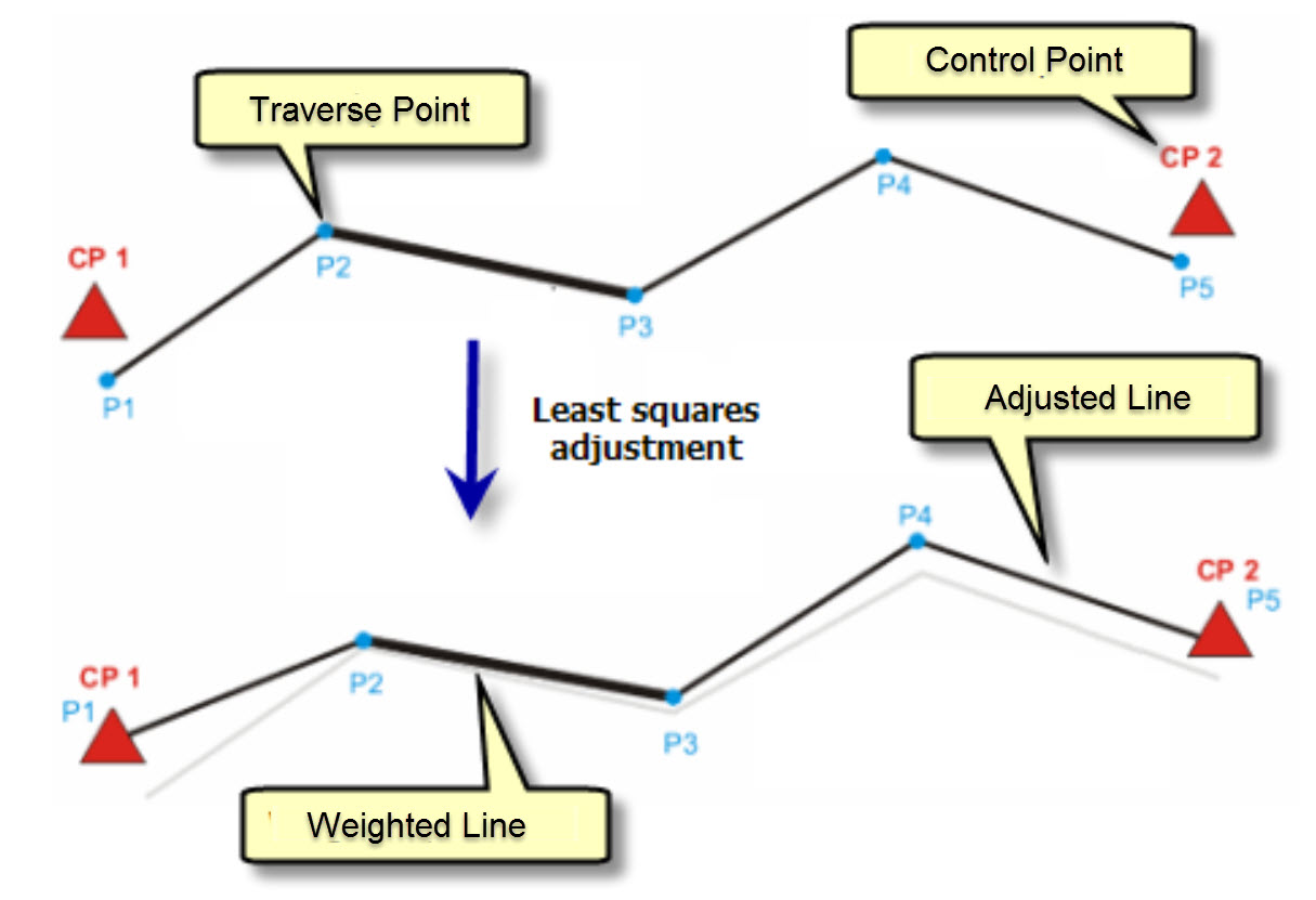
In QINSy weighting of observations is done through a priori SDs, primarily entered in the Database Setup program. Typically the manufacturer of each sensor provides accuracy figures, often in the form of standard deviations, which can be used for weighting of observations. Bear in mind that these are usually quite optimistic and may not be achievable in a survey situation, especially in less than ideal conditions. Combining manufacturer numbers with his/her own experience, as well as soliciting advice from other experienced professionals, the surveyor is able to reasonably estimate appropriate SDs for the current survey. These a priori SDs constitute the stochastic model. The smaller the SD value assigned by the surveyor the more weight is associated with that observation. The least squares network computation uses relative weighting in calculating best estimates for position. More heavily weighted observations are more constrained in the the degree to which their values can be changed during the least squares adjustment. Such constraint impacts the best estimate of position. The following diagram shows an example of weighting one traverse leg P2-P3 more heavily; the adjusted locations of P2 and P3 are constrained and have not shifted as much as the other traverse legs.
Statistical Testing
QINSy uses two statistical tests to check whether the actual observations and a priori SD’s used agree with the mathematical and stochastic models and to identify and reject outliers. Both statistical tests are based on the analysis of the least-squares residuals, which are the differences between the measured value and the least squares computed value. The F-Test is an overall model test and the W-Test examines each observation individually.
F-Test
The F-Test is a general test which tests the overall model. A failed F-Test indicates that there is a problem, but not what the specific problem is. The F-Test will fail if there is some outlier present in the network or if the network has a bad layout because of missing observations or loose ends, but also if the a-priori SD’s are too optimistic, i.e. if we think the observation is better than it really is and we have given it a heavy weight when it should have a lower weight. In this case the a priori SD value needs to be larger.
The critical value for the F-Test is computed using the so-called Fisher-distribution and depends on the number of redundant observations. In QINSy this value can be seen in the Computation Status Display. The F-Test will fail if the computed estimate of the variance factor after the least-squares adjustment (a-posteriori) divided by the adopted variance factor (computed from the a-priori observation variances) is larger than the critical value.
W-Test
The W-Test checks each observation in the network for a blunder against a pre-defined critical value. Because of the 1D nature of this test, it works particularly well for observations like directions, vertical angles and distances. For USBL observations and offsets, each element dX, dY and dZ is tested separately against the critical value.
The critical value for the W-Test is computed using the level of significance, which is set to 99% (100 --alpha %), and the power of the test, which is set to 80% (beta %) in QINSy to comply with the UKOOA Guidelines For The Use Of Differential GPS Offshore. In QINSy this value is 2.58 and can be seen in the Computation Status Display. The W-Test will fail if the test quantity is larger than the critical value. The test quantity is computed from the observation residual and its a-priori SD, so a large residual will not necessarily mean that the W-Test will fail.
Data Snooping
Data snooping is a process of successively checking the W-Test quantity of each observation against the critical W-Test value and removing the observation with the largest W-Test value as long as there is sufficient redundancy. In statistical jargon, this means testing a series of alternative hypothesis each of which assumes that there is an error in one observation if the null hypothesis is rejected. In QINSy, W-Test values can be seen in the Observation QC Display.
What Constitutes an Adjustable Network
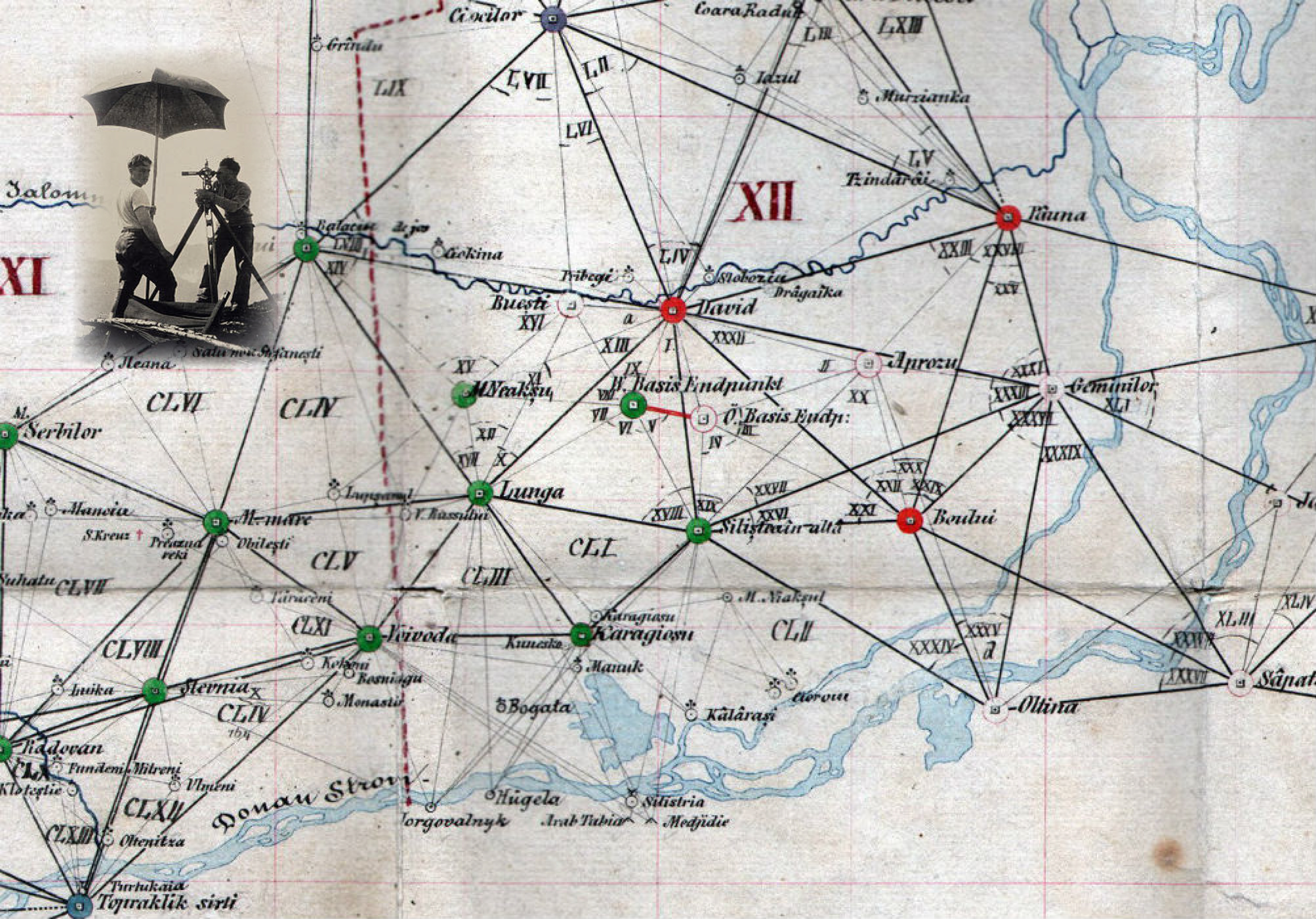
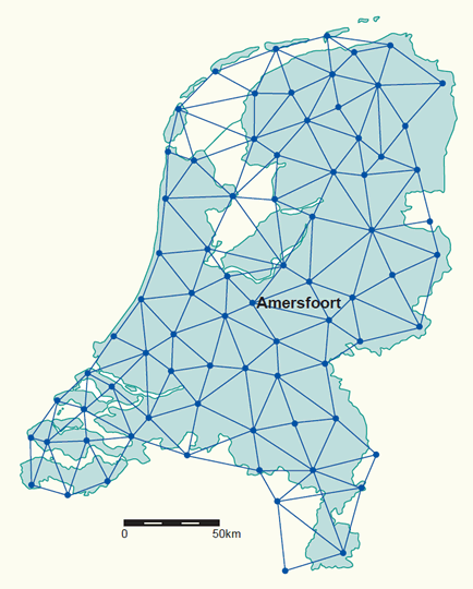
To appreciate the way computations work in QINSy it is useful to understand what combination of fixed and variable nodes, observations and offsets constitutes a network that can be adjusted and statistically tested using least squares? In this context the word 'Network' implies multiple nodes interconnected by multiple observations. Classically a network was formed by triangulating between multiple survey stations as, for example, in a country's geodetic control.
Old triangulation, Ingolstadt Germany |
Old triangulated Dutch geodetic network |
|---|
Many of the survey configurations in hydrographic survey do not qualify as true networks. Some have no internal checks and cannot therefore be subject to statistical testing. A few examples should make this clear.
Vessel positioning by Geodimeter
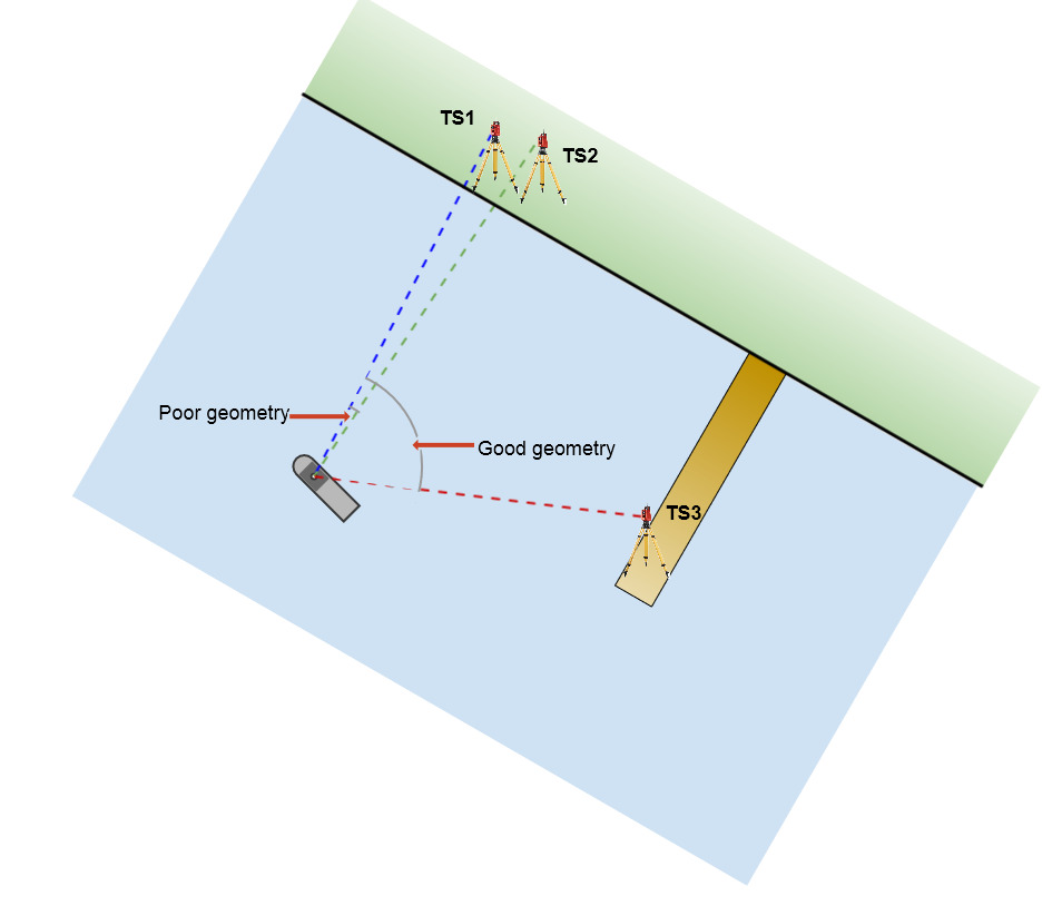
A single total station located at a known point ashore can use range and bearing measurements to track a target on a survey boat. However, relying on a single observation is risky because there is no way to tell whether the measurement is 'correct', and hence whether the computed position is 'correct'. A second range and bearing measurement from another known survey point will confirm, or check, the coordinates defined by the first measurement. If a second total station is installed close to the first total station there are now two ranges and two bearings providing a check on vessel positioning. Such an arrangement would establish redundancy but there would be very little 'strength' in the angle geometry of the network. It would be preferable to locate the second total station with a sufficient distance from the first that the angle of intersection at the vessel is greater than 30º, preferably 60-90º. Generally, the more measurements fixing the coordinates of a survey point, the more reliable the coordinates. These additional measurements are called redundant measurements. Good geometry gives the network 'strength'.
Simple Multibeam Setup
In light of the foregoing, a simple vessel set up with a single GNSS receiver, one motion reference unit, one gyro, one multibeam and measured offsets does not constitute a true network. The GNSS antenna position is the result of a true least squares network adjustment performed by the receiver, but there are no checks built into the configuration. Computation of seabed soundings is propagated from the GNSS antenna position through offsets oriented by pitch roll heave and heading observations to compute position of the multibeam head. The one way propagation of position continues to the soundings on the seabed, i.e. the propagated computation of position is one directional. If there was an error in an offset it would remain undetected until the cross checking of soundings. Bathymetry checks are made by examining swath overlaps, running cross lines, comparison with previous surveys and so on. With no redundancy statistical testing does not work in this situation.
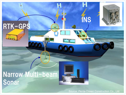
However, add a second receiver, and/or gyro, and/or MRU to the configuration and you have a network of sorts; the setup now has redundancy but no 'strength of figure'. The offsets measured between two GNSS antennas creates a constrained link that a least squares adjustment can test.
ROV Tracking
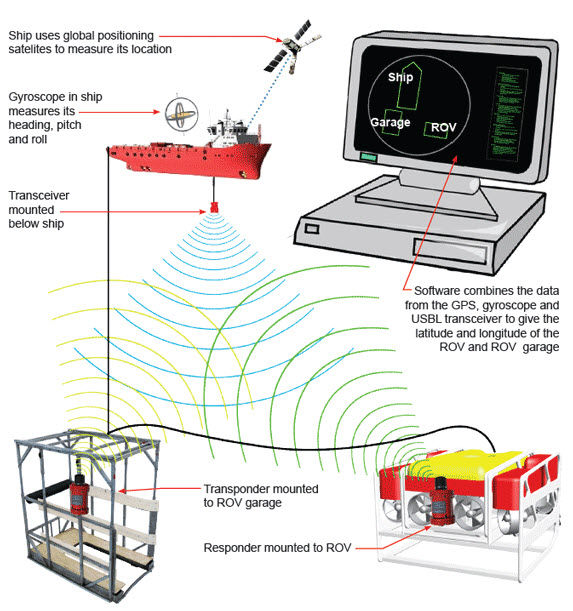
As with the simple MBE example, a minimal configuration for tracking an ROV would comprise one GNSS, one gyro, one MRU, one USBL system and one transponder mounted on the ROV. This too propagates the computation of position from GNSS antenna through offsets oriented by gyro and MRU observations to the USBL transducer and thence to the ROV transponder. If equipped with gyro and MRU, the one way propagation of position from transponder node to a second node through offsets oriented by gyro and MRU observations.
 |
|---|
Should two or more transponders be mounted on the ROV there is a check observation from USBL transducer to the ROV, but there is no check on the computed coordinates of the transducer.
If the ROV being tracked by USBL is also positioned through an acoustic long baseline spread, the configuration is a proper network with redundancy. Statistical testing is then possible.
Seismic Survey - a classic network
The typical configuration of a 3D seismic survey spread illustrates the classic network, exhibiting redundancy and geometric strength. In the image below dotted lines represent acoustic ranges measured between six seismic streamers, the guns (sound sources) towed immediately behind the vessel, the vessel itself and the six tail buoys. Additional observations include rGPS ranges and bearings from vessel to tail buoys, laser ranges and bearings from vessel to guns, multiple compasses mounted along each streamer, as well as the usual survey vessel sensors such as multiple GNSS receivers, multiple gyros and motion reference units. Offsets measured between the locations of the various sensors are also included in the computation.
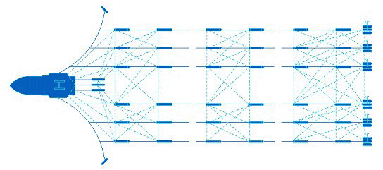
Of course the whole network hinges on the vessel position and orientation. This is not as risky as one would assume at first glance. The computation of GNSS positions is also a network comprising satellite 'base' stations, pseudorange observations and differential/RTK corrections. With five or more satellites received there is pseudorange redundancy and statistical analysis of computed positions is possible. Typically this network adjustment is done inside the receiver and final positions are delivered to QINSy. Most seismic vessels will carry two or more GNSS receivers, receiving differential corrections from different sources (WAAS, Omnistar, Veripos etc.). Therefore vessel positioning can be both accurate and reliable. Two or more gyros, plus computed heading between GNSS antennas provide accurate and reliable vessel orientation.
All these different observations (which can add up to hundreds) are included in one big least squares adjustment to yield the best estimated positions of the many hydrophone receiver groups embedded along the length of each streamer. The physical network is the mathematical model comprising all the nodes and observations. The stochastic model must be determined by estimating the a priori standard deviations (weights) of the different types of observations.
Rock dumping configuration
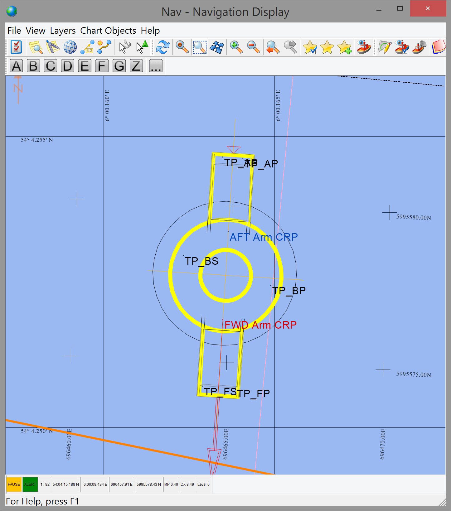
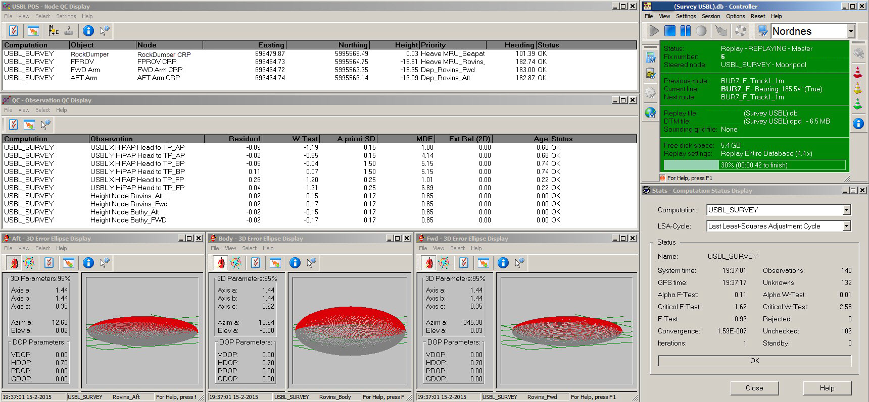
Some complicated construction survey configurations do take advantage of QINSy's statistical testing and support of multiple computations. For example positioning of a fall pipe on a rock dumping project often entails use of multiple instances of the same sensors, as well as multiple different sensors. It is not unusual to mount multiple USBL transponders, gyros, MRUs, INS, speed logs, and deptth/altitude sensors on the rock dumping vessel, on the fall pipe ROV (FPROV) and on the fore and aft arms that are hinged to the FPROV. The Navigation Display below shows the FPROV with fore and aft arms deployed. Six USBL transponders are mounted (TP_XX).
|
|
|---|
This full screen capture shows the best estimated positions in the Node QC, residuals and W-test values in the Observation Physics, statistics in the Computation Status, and 3D error ellipses.
Anchor handling configuration
In a multiple vessel survey configuration, such as anchor handling associated with pipe lay for example, there may be a danger in combining all vessels in one network adjustment. Typically in these situations, positioning of anchor handling tugs is quite independent of the pipe-laying barge and of each other. In other words there are no observations between the barge and tugs, or between the tugs themselves. By combining all in one computation a network dependency between objects (barge and tugs) is created when there is none in reality. The risk is that a breakdown in positioning of one object may, in theory, cause the computation to not solve or to crash. It may be wiser to create a separate computation for each object.
Multiple defined computations
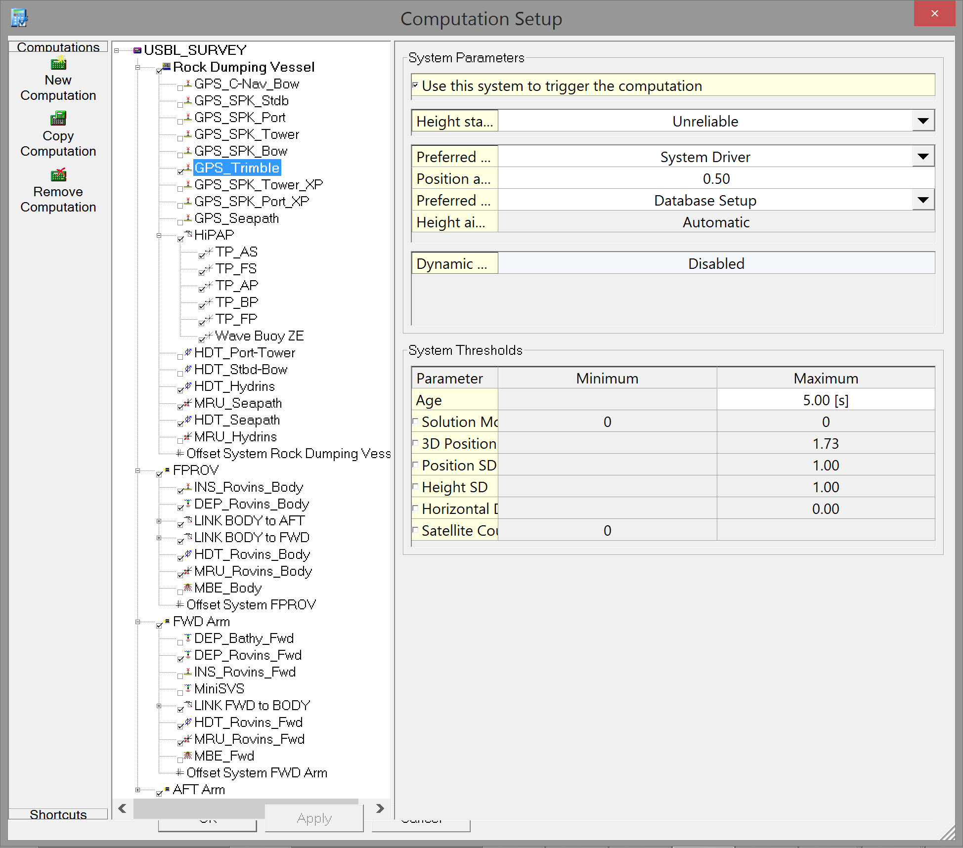
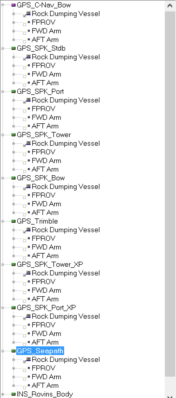
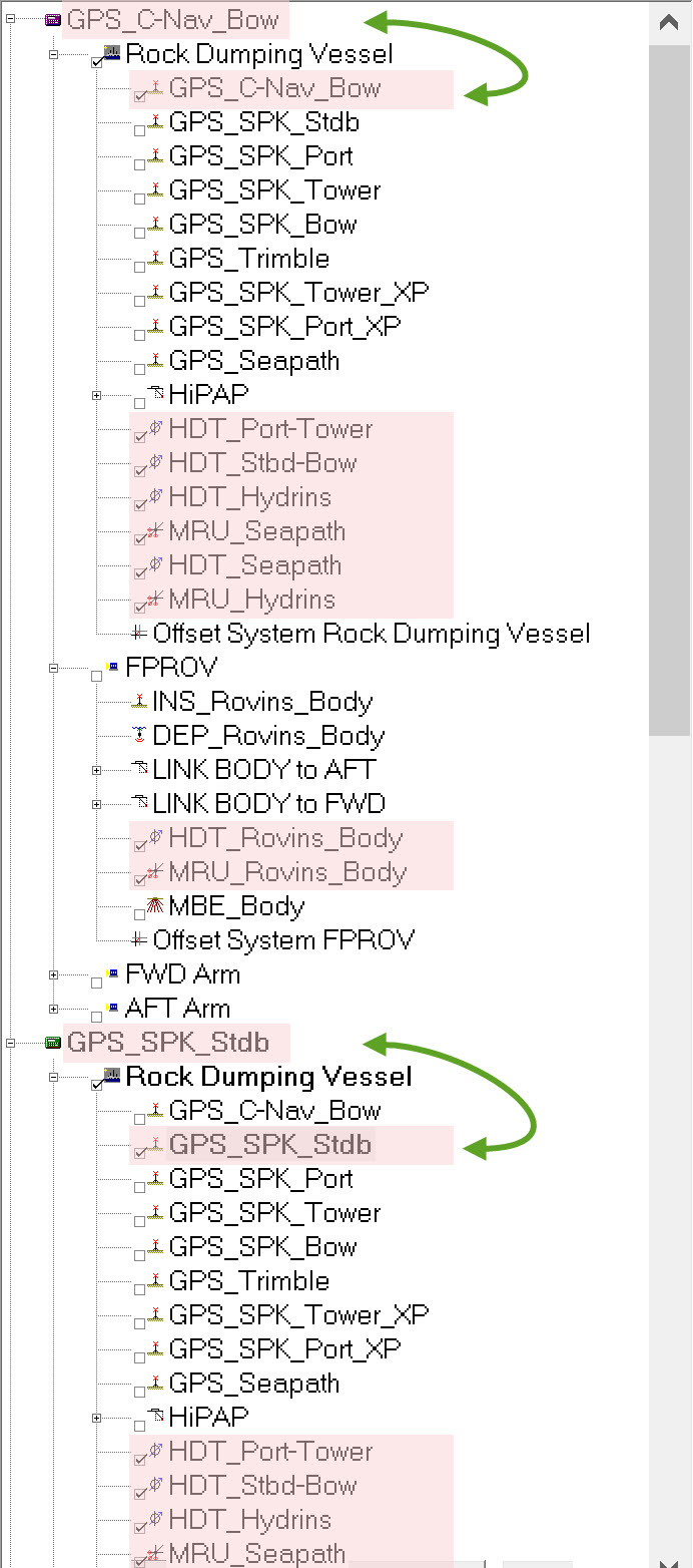
When first starting the Controller with a new template database QINSy will automatically define one computation for each position navigation system defined in the template database. By default the computation name assigned is the name of the positioning system defined in the template. For many surveys using a simple configuration with a single GNSS the one default computation is usually sufficient. In more complicated configurations like the preceding rock dumping example QINSy creates a default computation for each positioning system defined (graphic below left). Under the name of each computation all the objects, systems and observations are listed in the middle panel of the Computation Settings dialog.
When building a template database the main surface vessel is defined first. This is the object that is automatically enabled for each computation; in this example the object is called 'Rock Dumping Vessel'. The other three objects are not enabled; this task is left to the surveyor as work to define the final computation configuration proceeds.
Apart from the Position Navigation System, the only other systems automatically enabled on each object are the gyro and MRU systems. Note that initially only one object is enabled but that the gyro and MRU systems are checked for each of the other objects (highlighted in pink in the graphic below right).
Computation automatically created for each Position Navigation System |
Systems that are automatically enabled on each object |
|---|
Whether the surveyor wants to keep multiple computations running is a personal decision. What remains is for the surveyor to refine and complete each computation by enabling the appropriate objects and systems to be used in the computation.
There are instances where only one Position Navigation System is defined in the template, resulting in only one computation created automatically. However the surveyor is free to set up multiple least squares computations in order to provide further checks of positioning integrity. For example, if two GNSS are defined in the template, two computations are automatically created each with a single GNSS enabled. It might be interesting to compare the two computed results with a third computation in which both GNSS systems are enabled. The list of objects, systems and observations is repeated under the new computation name and you select which you want to activate. One computation can be compared with the another as a quality assurance check.
In more complicated survey configurations it may be desirable to define even more computations. For example in the seismic network example mentioned above, a second computation positioning the gun arrays just using the laser ranges and bearings might be compared to a third computation positioning the gun arrays just using acoustic ranges. It is always good survey practice to build checks into your configurations.
Or in the rock dumping scenario, several computations might be defined using different combinations of all the sensors. Each computation can be used as a check on another. Alerts could be configured to compare positions from different computations.
Guidelines
Computation Settings
Under Computation Settings in the Controller, various settings can be defined for each of the computations (least-squares adjustments) created, and, within each computation, for each connected Object and observation (or System) individually. Make sure to define realistic a-priori SD values in Database Setup. In QINSy the computation settings are used by:
- The PreProcessor
- DrvHeightAiding
- Adjustment
- PositionFilter
to determine which observations and nodes are to be used in the least-square adjustment and subsequent steps.
Computation Parameters
Computation Name
When going online for the first time with a template database, new computations are automatically added for each position navigation systems and/or satellite systems. By default the name of the computation is the same as the position navigation system name; but the surveyor is free to change the name. The computation name is visible in various displays so a short descriptive name is preferable.
Triggering System
Each update of the selected triggering system initiates a computation cycle that calculates positions for all of the unknown nodes in the adjustment. For example, if a positioning system with a 1Hz update rate is selected a computation cycle will be triggered once per second. Be aware that sometimes position is output at higher rates as, for example, in an integrated sensor such as a POSMV. If the motion data is setup to output at 100Hz (note >25Hz is not necessary), and the rate of position output as trigger is not reduced, QINSy attempts to cycle through computations at the same rate, i.e. 100 separate computations are performed 100 times per second. In addition to this not being necessary from a survey positioning point of view, CPUs are put under strain to the point that the entire system will slow down, or maybe even crash.
It is normally not necessary to trigger computations at a rate >5-10Hz.
At present, positions from other positioning systems are not skewed to triggering time!
Maximum Triggering Rate
Iteration Threshold
The least squares adjustment is an iterative process, starting with an approximate position and narrowing to a better estimate with each iteration. Rather than let the computation iterate indefinitely as when the network is complex or there is no convergence, the iterative process may be terminated by setting the maximum number of iterations. Normally only one iteration is required when there is no redundancy, e.g. in case of just a positioning system on one vessel. When using USBL systems or range/bearing systems, at least two or three iterations are required, so the default number of iterations (10) will never be reached. A higher value (20) might be necessary when towed objects are part of the network and/or computed heading or attitude is enabled.
Statistical Testing
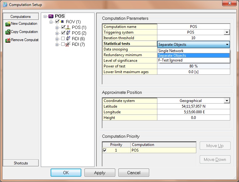
Statistical testing is a new computation setting that replaces some ‘hidden’ registry settings and automatic checks on bundle objects in Adjustment and PositionFilter. It also enables or disables the LSA cycles described above. The labels are short descriptions of the test options. They are only preliminary and may be changed in future releases.
- Single Network
Default setting for existing computations is the ‘single network’ solution. With this setting selected, the least-squares adjustment is only allowed to cycle once, i.e. only Step (1) is carried out as described above. The adjustment fails if the solution does not solve, does not iterate below its limit, or fails the F-Test (even if data snooping is enabled). Both the computation and the connected nodes will get a ‘bad’ status and the computed node positions are not used in the subsequent position filter step. However, if a previous adjustment trigger has been successful, the computation might go into (or stay in) prediction mode. Computation status can be seen in the Computation Status Display, observation statuses in the Observation QC Display, and node statuses in the Node QC Display.
- Separate Objects
Default setting for new computations is the ‘separate objects’ solution. In this case, the least-squares adjustment is allowed to carry out steps (1) to (3) as described above.- If the adjustment already solves in the first step, which will be the majority of the cases when the mathematical and stochastic models have been set up correctly, then the next steps are not necessary. All the objects will be computed, except for the objects for which there are not enough observations (less than three).
- If the second step succeeds, then the last step is not carried out anymore. In this case, only the objects connected to absolute position observations will have been computed.
- In the third step, all objects are computed independently and will only solve in case they have absolute positions.
- F-Test Ignored
The ‘F-Test ignored’ option is only to be used as a last resort if a computation is not solving because the F-Test fails. With this setting selected, the least-squares adjustment is allowed to carry out steps (1) to (3), and F-Test failures are ignored for both computation and node statuses. The position filter step will therefore continue to use the node results from the adjustment step. Be aware that an F-Test failure indicates a problem in the network setup. It is most likely that the computed positions will include a shift in coordinates if the test fails because of incompatible observations such as USBL dZ values versus ROV bathy depths that refer to a different height level. Instead of using this setting, it is advised to increase a-priori SD values or disable faulty or unlinked observations.
Data Snooping
Data Snooping (iterative W-Tests checks as described earlier), can be enabled or disabled. Default setting is that data snooping is enabled. If there are no redundant observations, then this setting will not have any effect.
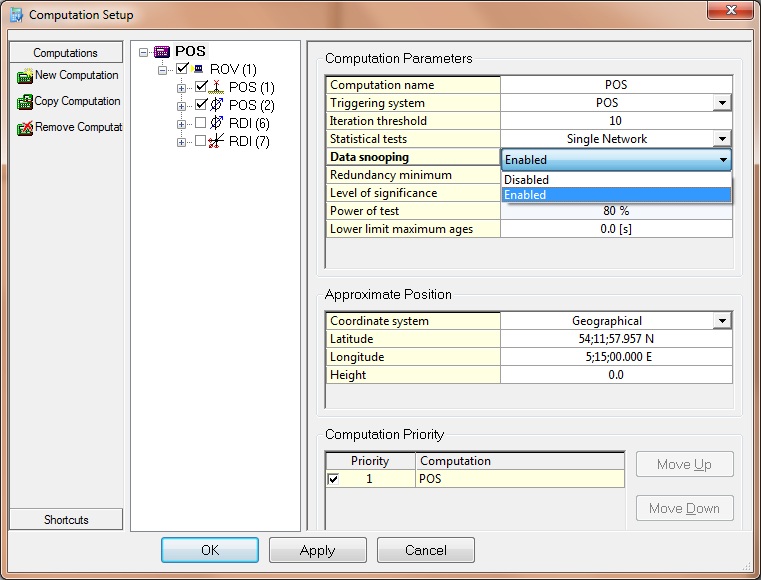
With data snooping enabled, the most likely erroneous observation (i.e. that with the largest W-statistic greater than plus or minus 2.58) is removed from the least-squares solution (with status ‘snooped’) and the remaining observations (and statistics) are recomputed. This process will continue while there is sufficient redundancy.
Data snooping is done in each of the adjustment Steps (1-3) described above, at the end of the iteration loop. If data snooping is successful, it can result in a successful adjustment and no further steps are carried out anymore.
The W-Test values for each observation in a computation can be seen in the Observation QC Display.
Redundancy Minimum
Redundancy or Degrees Of Freedom (DOF) is the number of observations minus the number of unknowns in a least-squares adjustment. A minimum number of redundant observations of one is required for statistical tests. If data snooping is enabled, the rejection of observations may only continue until the minimum number is reached.
Statistical Test Parameters
Level of Significance has been set to 1%, and Power of Test has been set to 80% to comply with the UKOOA Guidelines For The Use Of Differential GPS Offshore.
These parameters are fixed (depending on registry key).
Lower Limit Maximum Ages
A lower limit on the maximum age of all observations in a computation is imposed if this parameter is not set to zero. The lower limit is also used for the position rejection age of connected objects. Since some observations such as object priority settings for attitude and height are common for all computations, this limit could have a significant effect on other computations. If limit is reset to 0, maximum age settings are not checked (but also not altered).
The lower limit may be either 0 (disabled) or between 5 and 60 seconds. Higher maximum ages may be set for individual observations. If a non-zero lower limit has been set, and some maximum age in the computation is changed to a value less than this limit (but larger than 5 seconds), then the lower limit is corrected to that value.
Approximate Position
In earlier QINSy versions
- GNSS Systems
A good approximate position was required in order for a computation to work correctly. For positioning systems, a position on the same continent was good enough. - For range/bearing systems
Such as a total station, the approximate position had to be very accurate, i.e. on the correct side of the station node.
- GNSS Systems
In current QINSy versions
- GNSS Systems
All nodes in a computation are shifted to a new approximate position, if latitude and longitude from a positioning system are found. - For range/bearing systems
The object on which the ‘at node’ is located, is shifted to a position in the direction of the bearing observation (using an approximate range of 50 m). - Thus QINSy now determines its own approximate positions and this setting is not so important anymore.
- GNSS Systems
Computation Priority
The priority of the different computations determines which computation results are used for output node positions and echosounder footprints. When looking for an output node or an echosounder system, QINSy searches the priority list for the first computation in which the node or system has got a valid position. Likewise, the first computation in which a computed object is found (which also does not necessarily have to be the top priority computation in the list) is used to populate the results buffer.
The highest priority computation is indicated by a magenta icon in the tree list. Other active computations are marked by green icons.
Computations that are on standby (also being computed so that they don’t have to be initialized before being set to active) are indicated by grey icons.
Disabled computations are shown with a red icon.
A computation status can be set to 'Enabled', ‘Standby’ or ‘Disabled’.
The computation priority is also important when using the RTK height as tide.
Read the next document when this applies to your project: How-to Use/Setup RTK Tide.

