This document describes how to interface, use and process data from Sidescan Sonar systems.
Info
To use SSS in Qinsy, the Side Scan Sonar Support Add-On is needed.
Sidescan Sonar (SSS) is a device that measures the intensity of the reflections from the seabed or objects on the seabed. SSS is usually towed approximately 10% of the sonar operating range elevation above the seabed.
There are also multibeam echosounders capable of outputting data in two channel SSS format or singlebeam echosounders that have a SSS add-on. A SSS can be operated from another object (tow fish) or it can be mounted on the survey vessel or an underwater vehicle (ROV/AUV).
On this page:
In short the workflow is as follows:
Add the Sidescan Sonar as a system to your setup. Possibly a depth recorder and an altitude determining system need to be added as well when the sidescan sonar will be towed behind your vessel. This then also requires a layback definition.
Activate the available systems. Activate the correct sounding grid and DTM files to record the data. The raw sonar data packets are stored in *.db files and the vessel and footprint positioning data are stored in *.qpd files. Set up the Sidescan Image Display to view the data while recording.
Load the data into the Survey Manager and use the Sidescan Viewer tool to review the data. Create a database of targets found with the Sidescan Viewer and use the Target Viewer to view and edit the targets. (See bottom of page.)
Setting up a SSS system in Database Setup
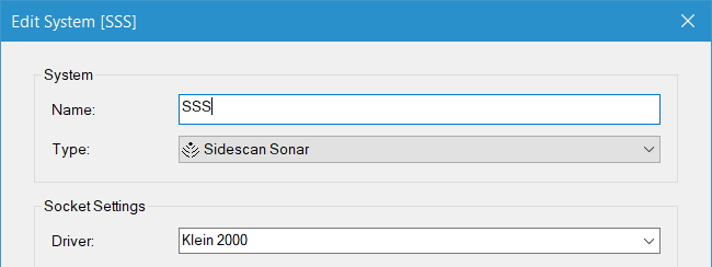
Create a New System in Database Setup on the Object on which the SSS is installed:
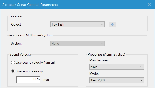
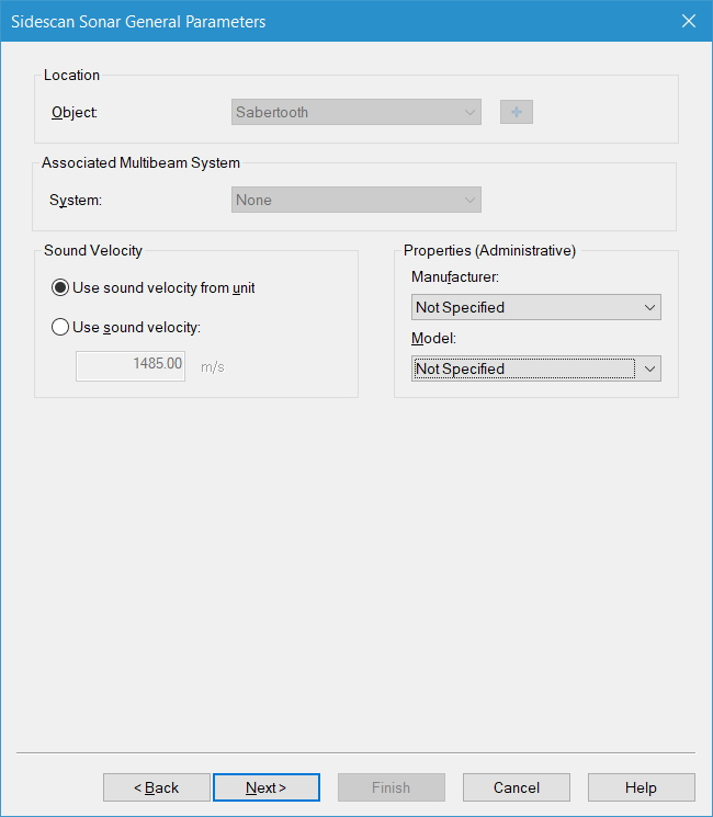
The second page contains the General Parameters:
Sidescan Sonar General Parameters
Location
Object
From the drop down menu select the Object on which the system is located.
Associated Multibeam System
System
In case the Sidescan sonar is an add-on system to a Multibeam system, select the originating Multibeam system here.
Sound Velocity
Use sound velocity from unit / Use sound velocity
If the unit does not have a real-time Sound Velocity System, select "Use sound velocity" and enter a manual sound velocity to be used.
Properties (Administrative)
Manufacturer / Model
These items are for administrative purposes only and will not be used by Qinsy for computations or data correction
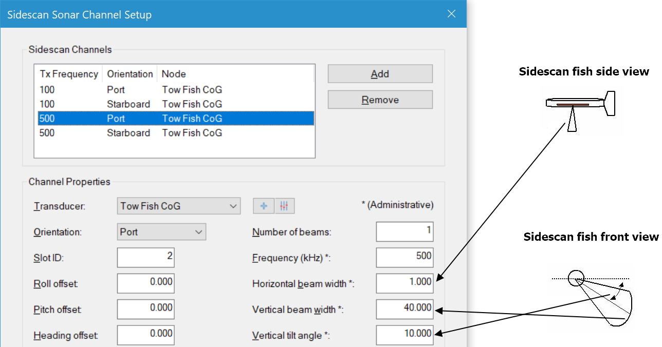
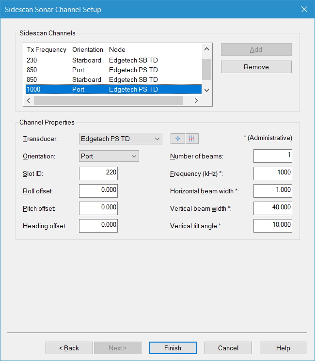
The third page contains the Channel parameters:
Using the Channel Properties, set the appropriate Transducer, Orientation and Offsets. The other items are administrative (not used by Qinsy for computations or data correction).
Sidescan Sonar Channel Setup
Sidescan Channel(s)
Use the Add button to add the Sidescan Channel(s).
Channel Properties
Transducer
Node at which the transducer or channel is located. For a Multibeam Add-On Sidescan both channels usually share the same node as the originating multibeam system.
Orientation
Direction to/from which the transducer is transmitting/receiving.
Slot ID
Depending upon the selected SSS interface driver, some require the SLOT ID to be entered to allow Qinsy to decode multiple channels of SSS data. An example is a dual frequency SSS unit providing 4 channels of data (2 channels per frequency). Refer to the Qinsy Drivers and Interfacing manual for further details. The Slot ID is not used for local area network ID.
The GUI is sensitive to the chosen device driver - in the case only two channels are available, no SLOT is shown. In the case of a dual frequency SSS then up to 6 channels can be declared and SLOT numbers are required.
Roll, Pitch, Heading offsets
Mounting angles of transducers (same as with Multibeam systems). Note that roll value is ignored since Sidescan is by nature indifferent to roll.
Number of beams
Always set this to 1 except when using a Multibeam Sidescan sonar system like Klein 5000 Series.
Note
In case of a Multibeam Add-On Side Scan (e.g. the Sidescan option of an 8125 or 8101) always set this to 1 and not the number of beams of the Multibeam transducer!!
Frequency (kHz)
Nominal transmitting frequency.
Horizontal beam width
Opening angle of transducer in horizontal direction (usually 1-2°).
Vertical beam width
Opening angle of transducer in vertical direction (usually 40-60 °).
Vertical tilt angle
Angle between horizontal axis and center beam limits (see figure above).
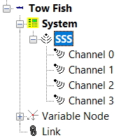
EXAMPLE: Edgetech triple frequency SSS (6 channels, 2 on each frequency)
Pressing “Finish” will close the setup of the System and will save the changes.
A new Sidescan system appears in the tree view below the Object, see figure below. A glossary of the properties of either system or individual channel can be viewed in the right pane of Database Setup when a tree item is selected.
Info
Beam Widths and Angles are currently not used within Qinsy but are only used to export to Reson 6041 software.
Online
Computation Setup
After completing the Setup, the system can go online. Here the settings need to be entered in order to control the data that is coming in and to control the storage.
The Survey Manager and the Sidescan Viewer rely on the positions/altitudes of the sidescan sonar that are stored in the QPD so make sure that QPD’s are created and that the sidescan sonar is enabled in Computation Setup and Session Setup. Furthermore the SSS image can be displayed in various displays.
Enabling systems
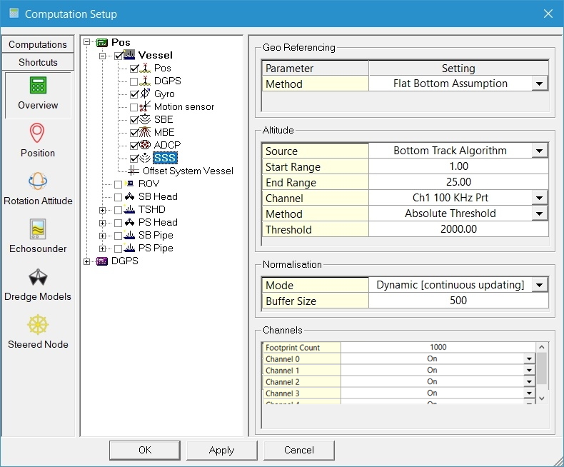
The parameters of the SSS can be accessed via the Computation Setup:
Make sure the Sidescan system is enabled in the Computation Setup.
Geo Referencing
Method
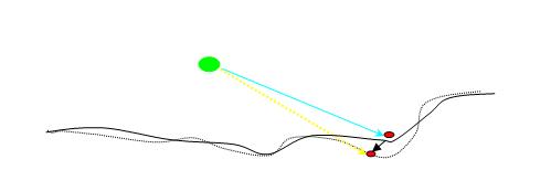
To locate the derived position from a beam, an assumption has to be made about the seabed. There are two options:
Flat Bottom Assumption All returns are located as if the seabed were flat. A radial distance from the SSS head is projected on a flat seabed, see figure below.
Flat Bottom Assumption
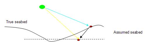
Sounding Grid The returns are projected with reference to a sounding grid previously filled, see figure below. Select the Grid layer that will be used for geo referencing.
Sounding Grid Reference
Note: the beam is now located lower than the flat seabed assumption. The radial distance is rotated to previous seabed displayed by the sounding grid. The elevation of the Sonar head is crucial in this assumption; an external observation is needed and only with RTK mode or tide corrected data a good result will be achieved. This can be done in Replay mode if tide data is not available online.
Altitude
The geo referencing of Sidescan data requires a proper altitude of the Sidescan fish above the seabed. The altitude is used to slant range correct the recorded data.
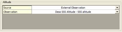
Source
The altitude source can be an External Observation system, e.g. an echo sounder or sensor in the fish:
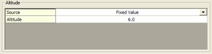
Or a Fixed user defined value:
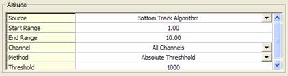
Or from a Bottom Track Algorithm. The bottom-tracking algorithm will try to detect the first bottom return from a Sidescan sweep. The assumption is made that the first strong reflection after the water column is the return from the bottom straight below the fish.
The algorithm will start searching at the sample represented by the search Start Range and searches up to the sample that is represented by the search End Range. When it finds the first sample that passes a certain Threshold (either user defined or calculated) then the algorithm will assume that the bottom is found at this sample. The sample number can be calculated back to a range with the Sidescan range and sound velocity value. The threshold will be, depending on the method, an absolute user defined value or relative to the swath's average or peak amplitude value. The algorithm detects the altitude for every individual channel and will compute the mean altitude afterwards.
Finally the altitude is filtered before it is accepted by the system. The last 15 pings are used to determine the mean altitude. Checking the ping altitude against the standard deviation rejects outlying altitudes. Currently we use a rejection threshold of 2 seconds. These values are hard-coded and cannot be changed.
Bottom Track Algorithm
Bottom Track parameters can be entered in the Controller (here) and in the Sidescan Image Display-Select-General (with “Use Altitude / Filter Settings from Controller” disabled).
Start Range
The Bottom Track Algorithm will start searching the samples for the bottom at this range. This can optionally be used to ignore the send pulse that may be visible in the data. This value may be left at zero if no apparent send pulse is visible in the samples. The value of the start range is in survey units.
End Range
The Bottom Track Algorithm will stop searching the samples for the bottom at this range. This constraint is put in to limit the amount of processing time. The value of the end range is in survey units.
Warning
If the actual bottom resides outside this gate then it will not be found!
Channel
If for any reason one of the channels is not working properly, or for example there is a jetty on one side, you may want to exclude that channel from the algorithm. You can make a choice which of the channels will be used to calculate the seabed.
Method
The threshold value can either be fixed or recomputed for every ping (relative). Which method works best for a specific system depends on the system characteristics, bottom type and bottom type changes during the survey.
The different settings are described below:
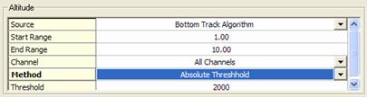
The user can define an Absolute Threshold value from 0 - 65535 (Amplitude range). The search algorithm will search through the sidescan amplitude samples and detect the bottom as soon as the sample value rises beyond this value.
Method: Absolute Threshold
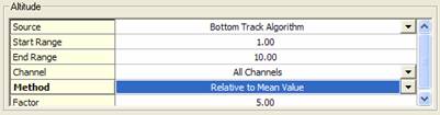
The threshold is re-determined for every new Sidescan ping. The Mean Value for the entire channel is computed. The threshold is then determined by multiplying the found mean amplitude with the Factor.
Method: Relative to Mean Value
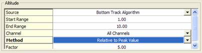
The threshold is re-determined for every new Sidescan ping. The Peak (maximum) Value for the entire channel is computed. The threshold is then determined by multiplying the found peak amplitude with the Factor.
Method: Relative to Peak Value
Example Klein 2000
Info
Disable normalization filtering when you fine-tune the bottom tracking parameters. The normalization will always start the amplification at the altitude range so even though the altitude is wrong it may still be ok to use because the normalization process will amplify the water column.
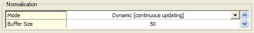
Normalisation
Mode
Dynamic (continuous updating) means normalization is switched on.
Buffer Size
Available when Dynamic mode is on. The signal from the SSS can experience some noise. The normalization mode (see figure above) removes noise by averaging a certain number of swaths (buffer size) in the buffer. The larger the value, the more noise reduction is applied. The normalization must be fine tuned so that buffer size is as low as possible but high enough to filter the noise.
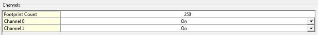
Channels
Footprint Count
This feature sets the number of virtual footprints. For these footprints an Easting and Northing are created and they will be stored in the sounding grid.
Make sure this number of footprint count enables a good topography of the bottom.
Channel x
Channels can be turned on or off in the Computation Setup. This means that they will not be stored in the QPD or the Sounding Grid, but they will be stored in the database.
Storage
The SSS data can be stored in a specific Sidescan data layer in the Sounding Grid for further processing. (Storage - Sounding Grid) The position and altitude of the SSS data can be stored in a QPD so that it can be loaded with the corresponding recorded database in the Sidescan Viewer tool. (Storage - DTM)
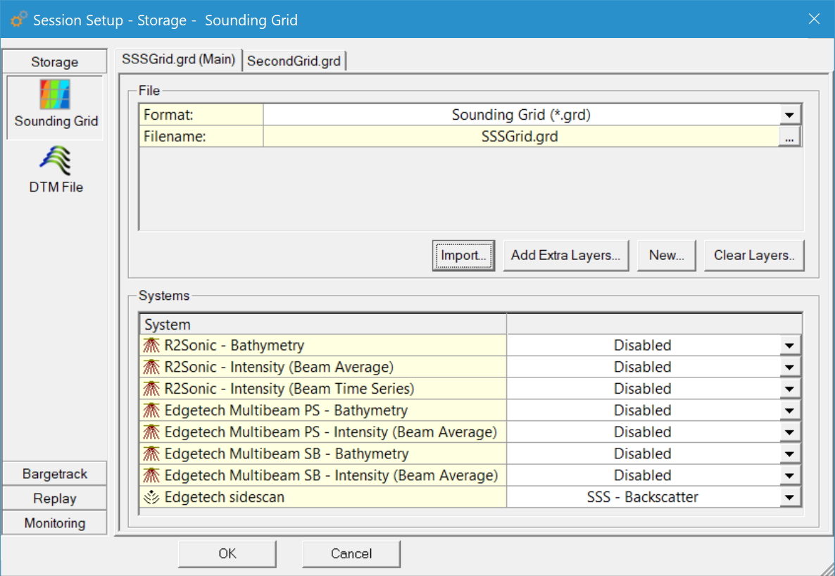
The storage of the sidescan data is done through Session Setup. Go to “Settings” on the menu bar and select “Session Setup”, the following dialog will appear:
Session Setup - Sounding Grid
Go to the Storage menu and select “Sounding Grid"
In the Sounding Grid menu select a grid using the browse button [ ... ]
For each System the Layer needs to be specified in the lower pane. (Use the button 'Add Extra Layers' when necessary.)
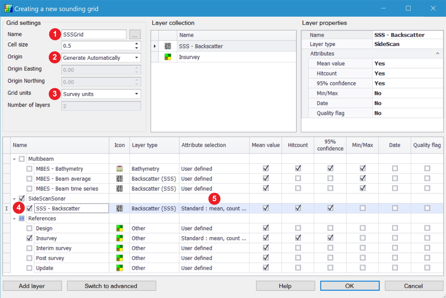
You may want to create a new grid to store the SSS data in. Carry out the following steps to accomplish this:
Press the 'New' button and the following dialog will appear:
Enter a file name and enter a base cell size. The size is dependent on the footprint count (see Channels): the higher the footprint count the smaller the cell sizes that can be used.
Select whether the origin of the grid must be generated automatically or that it must be specified by a grid Easting and Northing.
Select the unit type.
Select one of the layers in the lower pane and click on the 'Layer type' to select the correct one. The Icon will be adjusted automatically.
Click on the 'Attribute selection' and select which attributes to show. The more attributes are selected, the larger the sounding grid will be.
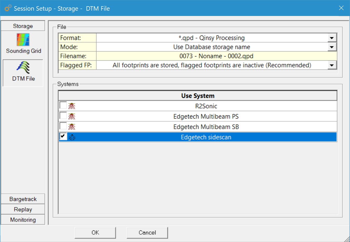
Session Setup - DTM File
In “DTM File” the format must be set to *.qpd. This will create result files which in combination with the raw database can be viewed in the Sidescan Viewer.
DTM Format should be set to *.qpd
Make sure the Sidescan System is enabled in the lower pane.
The Altitudes (e.g. from the bottom track algorithm or external observation) of the sidescan fish channels are stored in the QPD. These can be visualized and edited in the Sidescan Viewer.
Online displays
Sidescan data can be viewed in various different displays.
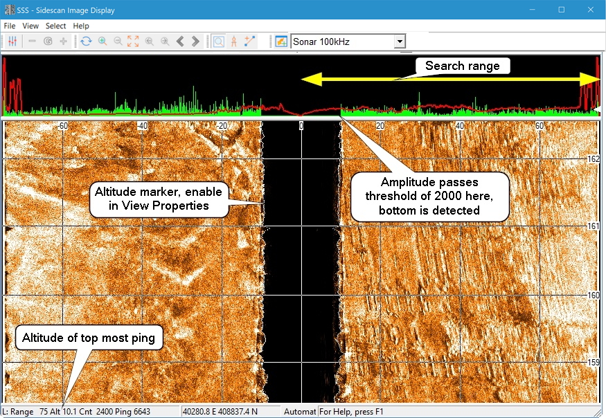
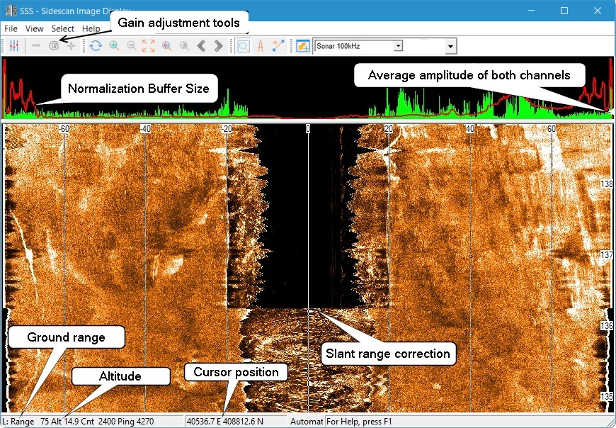
Sidescan Image Display
The Sidescan Image Display displays the conventional sidescan image digitally (see figure below). It displays the intensity of reflections from the seabed.
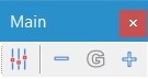
During recording the gain can be adjusted using the Main toolbar: Press the "G" for Automatic Gain, or press the + or - buttons repeatedly for manual adjusting.
With the slant range corrections switched on, the near beams are placed right underneath the sonar head. The water column will not be shown anymore. This will not affect the raw sidescan data. The sign on the right of the window (tiny white triangle) shows the average value for both channels. With Normalization On, data is transferred to fit this average giving a better view. This TVG (transmit variable gain) is set with the buffer size.
System Settings
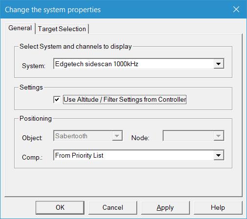
To enter the system properties go to “Select” on the menu bar and choose “System”. The following dialog will appear:
General system properties
In this window the system can be selected for display in the Sidescan Image Display. The settings which can be selected are those which are defined in the Database setup.
The Settings for Altitude and Filter can be changed in the Controller-Computation Setup. To change these settings in this window, remove the tick and the window will show two more tabs for these items. The settings from this menu will not be automatically copied to the Controller so either use this menu or the Controller but do not mix them.
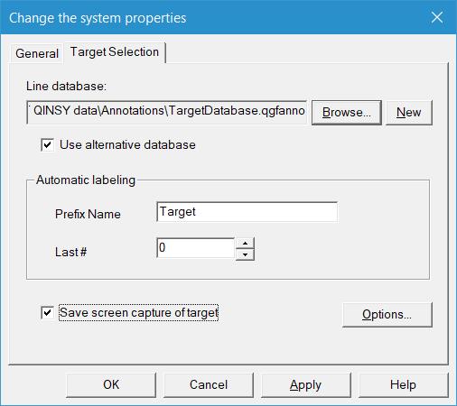
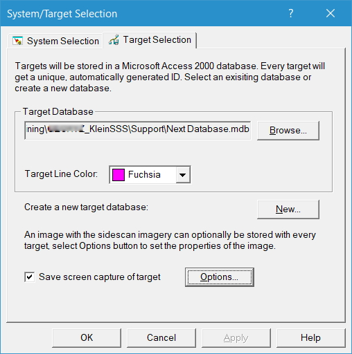
In the “Target Selection” tab (see figure below) targets will be stored in a *.qgfanno annotations database and also screen captures can be made of the concerning target.
Target Selection
The default storage location for targets is the Annotations.qgfanno file in the Project\Annotations folder, but when the option “Use alternative database” is selected a different line database can be used. The targets will be automatically labelled with a prefix name and number.
To save the targets' screen captures as bitmaps select “Save screen capture of target”. Press “Options” to open the Target image options dialog where the storage options can be set (see figure below).
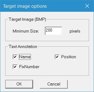
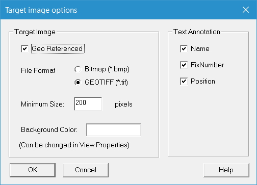
Target Image options
The target images are by default stored in the Project\Graphics folder.
During recording save a target as follows:
Go to “View” on the menu bar and select “Mouse Mode”
Select “Create New Targets” or press the 'New Targets' button in the toolbar.
Draw a line around the target in the display and use the right mouse button menu to save the target.
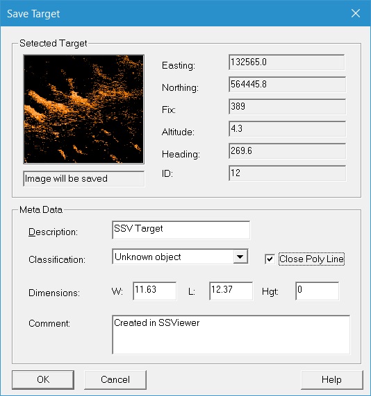
The following dialog will appear:
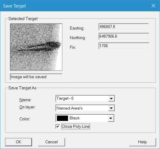
Save Target
This target is saved to the line data base file under Annotations as selected in the Target Selection menu above. The screen capture of the target is saved in the sub-folder Graphics.
Info
The Sidescan Image Display has its own F1 inline Help files to explain the functionality of all available buttons and options.
Navigation Display
Because the SSS data can be stored in a sounding grid it can be displayed in the Navigation Display. In order to display a sounding grid in the Navigation Display one must be selected in Session Setup (see figure Session Setup).
Go to “Layers” on the menu bar and select “Sounding grid”. The following dialog will appear:
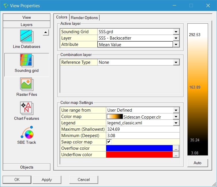
Sounding grid View Properties
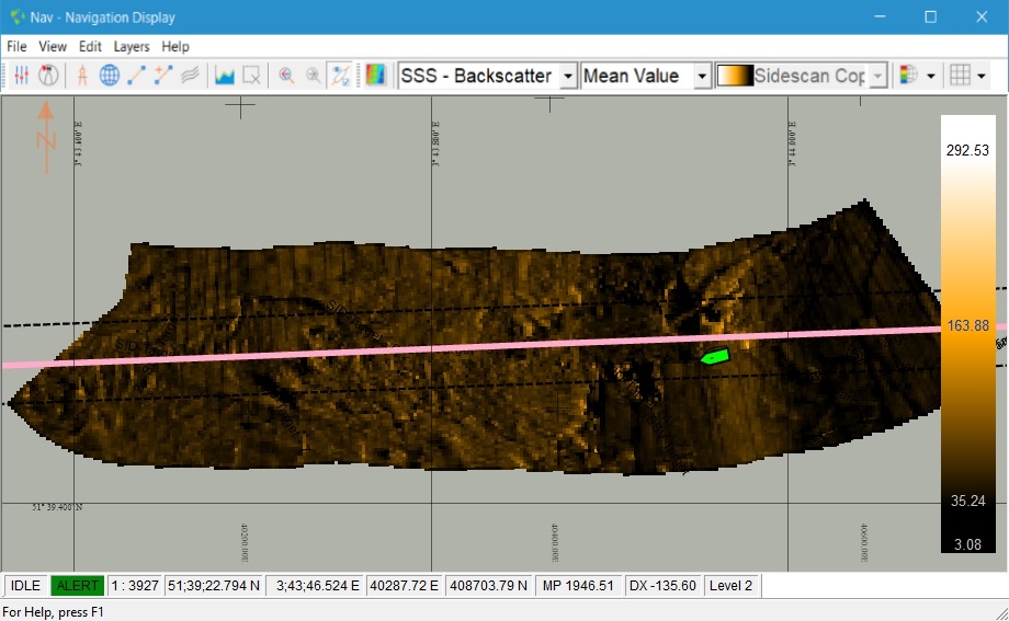
Select the correct Layer and the Attribute to show. Qinsy contains a specific Sidescan Copper color map that can be used to display the SSS data.
The following picture can be the result of SSS data displayed in the Navigation Display:
SSS data in the Navigation Display
It is possible to generate shade from a different layer and combine it with the Sidescan sonar image.
To enable this set the Sidescan sonar layer as Active layer.
Select the Render Options tab
For Render Grid select "Sun illuminated" or "Gradient & Sun"
For Shade Layer select a layer with depth information (DTM)
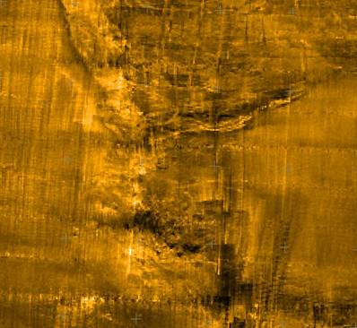
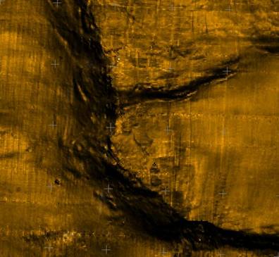
The difference between using shade or not is shown in the figures below:
SSS Gradient Colors (without shade layer)
SSS Gradient & Sun (with shade layer)
The first figure shows a normal Sidescan image; the second figure is a combined image of Sidescan sonar data and a DTM surface (for example multibeam data), providing more contrast.
3D Grid Display
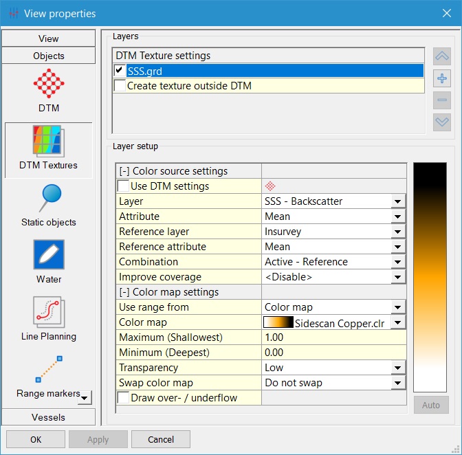
The 3D Grid Display is also able to display SSS data in combination with a DTM surface (for instance multibeam data).
To enable this option set "Layer" in the "Color source settings" pane to a layer that contains Sidescan sonar data or magneto meter data and select which attribute of the layer to show. To display differences between two grids a Reference layer can be used. Select the layer's attribute and the Combination mode.
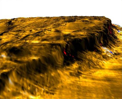
An example of a combination of SSS data and a DTM surface in the 3D Grid Display is shown in the figure below.
SSS data in combination with a DTM surface
Processing
As mentioned before the SSS data will be stored in QPD files and in a Sounding Grid file.
Survey Manager
Start the Survey Manager to be able to edit the Sidescan data.
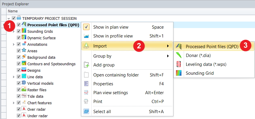
In the Project Explorer, right-click on Processed Point files (QPD)
Select Import
Select Processed Point files (QPD)
A regular Windows dialog will open where you can select the sidescan *.qpd file(s).
If you don't see the survey line(s) in the Plan View after pressing 'Open', press the 'Zoom to fit' button to make them visible.
Sidescan Viewer
Launching the Viewer
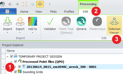
In the Project Explorer, select the QPD file(s) that contain(s) the track of the object on which the SSS is located, the SSS data is read from the corresponding DB file.
Press Edit in the Processing ribbon tab to access the processing tools.
Click on the Sidescan Viewer icon.
Multiple Sidescan Viewers can run at the same time as long as different files are selected.
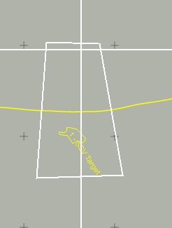
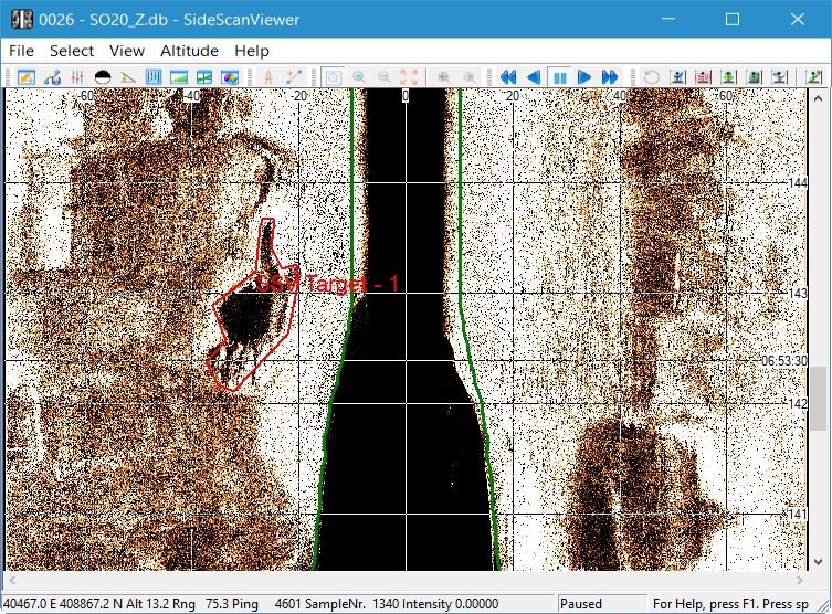
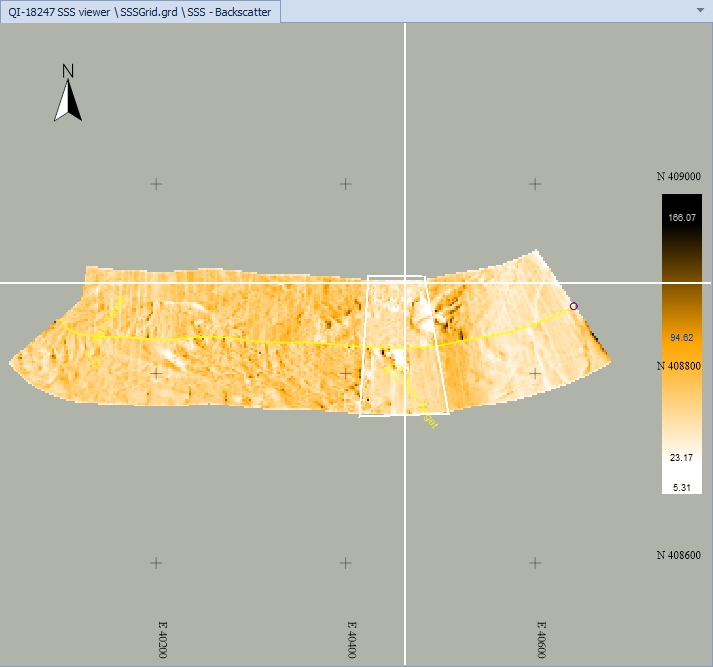
The Sidescan Viewer shows raw SSS data in combination with result data. The Sidescan Viewer is accessible either from the Qinsy Console via Replay, or from the Survey Manager via the Processing Ribbon Tab. The latter has the advantage that the view port extents are visible in the Plan View:
Viewport as visible in Survey Manager
The SSS data can look as follows:
Sidescan Viewer
The Sidescan Viewer has almost the same options as the Sidescan Image Display, but because it is a processing tool there are some extra options:
Normalization
In the Sidescan Viewer it is possible to use normalization. With this option it is possible to calculate and to apply a gain curve for each channel from the average intensity of both channels.
Before normalization the altitude must be applied correctly by a fixed value, an external device or with the Bottom Track Algorithm. The altitude settings are the same as used online (see Altitude).
To use normalization carry out the following steps:
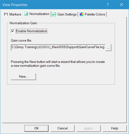
Go to “View” on the menu bar and select “Normalization Settings”.
Select the tab “Normalization”, the following dialog will appear: Normalization
Select “Enable Normalization”. Select “New” in order to calculate new gain curves.
In the appearing dialog select “Next” to continue.
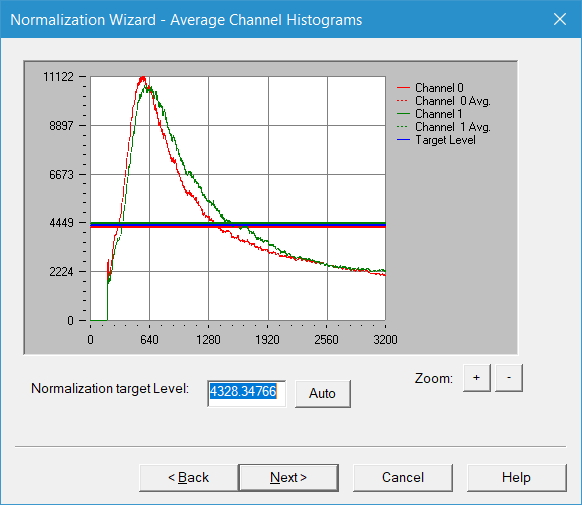
Select whether the normalization must be applied to all swaths or only the visible swaths. Select “Next” to continue, the following dialog will appear:
Average channel intensity
In the histogram displayed in the figure above the intensity and average of each channel are displayed, as well as a combined average. With this data gain curves will be calculated for each channel. The normalization module will automatically calculate a “Normalization target Level”. This can be adjusted manually if necessary.
Select “Next” to continue, the following dialog will appear:
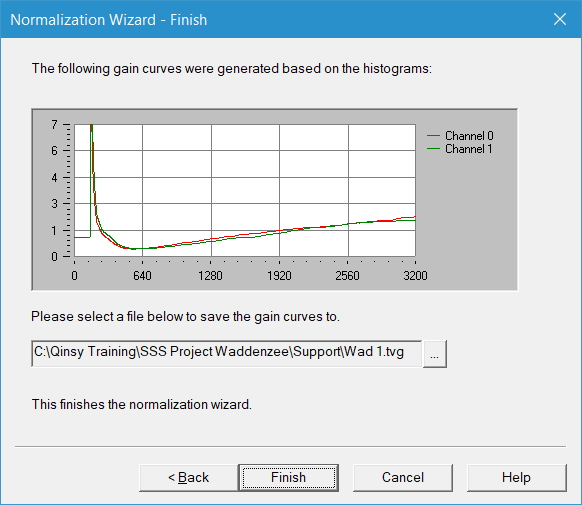
Gain curves
The histogram displayed in the figure above shows the calculated gain curves for each channel.
To save the gain curves to a file press the Browse button [ ... ] and specify a path. These gain curves can also be used for other SSS data that is viewed in the Sidescan Viewer. These files must then be selected in the “Normalization” tab of the “View Properties”.
Target Creation
In the Sidescan Viewer it is possible to save targets from the Sidescan image to bitmap or geotiff images.
Both image formats can be saved as geo referenced images. This means that the created image will have the correct coordinates of the target. In order to create these images follow the next steps:
Scroll to the position in the Sidescan image where the target is located.
Go to “Select” on the menu bar and select “Target Selection”.
Under the “Target Selection” tab, the following dialog will appear:
Target Selection
Select a target database using the 'Browse' button. If no previous database exists, use the 'New' button to create one.
Select “Save screen capture of target” and press “Options”. The following dialog will appear:
Target image options
Select whether the image must be geo referenced and what kind of file format should be used. (Only *.tif files can be imported for display in the Survey Manager.) By default the image files will be stored in the Graphics folder of the project.
Select the minimum number of pixels and the mask color. The mask color is the color that will be used on places where there is no data. Choose white for then best results in the Survey Manager.
Text annotation can also be added to the image, select the items of interest and press “OK” to finish.
Press “OK” to exit the “Target Selection”.
Go to “View” on the menu bar and select “Mouse Mode”, and then “Create New Targets”.
Click lines around the target and click on the right mouse button and select “Save Target”. The following dialog will appear:
Save Target
As can be seen, the image will be saved with an Easting and Northing coordinate.
The name of the image can be changed by typing in a new Descrition. A Classification name can be selected using the drop down menu. Classifications can be created in the Target Viewer tool, see below.
The image will be saved in the Graphics folder of the project, the lines drawn around the target will be saved in the Annotations folder and the target data will be stored in the Support folder.
Info
The Sidescan Viewer has its own F1 inline Help files to explain the functionality of all available buttons and options.
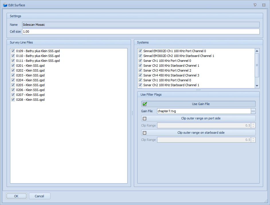
Side Scan Mosaic
Open the Survey Manager from the Console.
Go to File New, build a new Sidescan Mosaic, ensure to select the right systems and files to be used for the mosaic build and apply the gain file.
Ensure to select the Sidescan Mosaic in Project Explorer and change the color map if wanted.
Sounding Grid
As mentioned in Online - Storage the Sounding Grid can be filled with SSS data. The data needs to be imported into the Survey Manager to view it in the Plan View.
In the Project Explorer, right-click on Sounding Grids and select Import to select the recorded grid file.
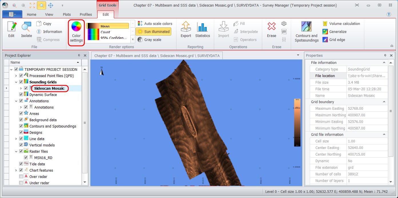
SSS data in a sounding grid in the Survey Manager's Plan View
Because a layer is used especially for SSS data the color map can be set to “Sidescan Copper”. This can be altered in the “Grid tools” tab - Color settings option.
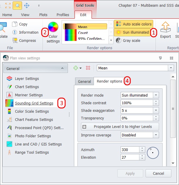
Sidescan data is backscatter data, so there is no height information available. To add shade for better contrast:
Press 'Sun Illuminated' in the Grid tools tab - Edit menu.
To adjust the Sun Illuminated settings go to the Color settings option
Select Sounding Grid Settings
Select the Render options tab. The shade can be adjusted by changing the “Azimuth” and the “Elevation” of the imaginary light source.
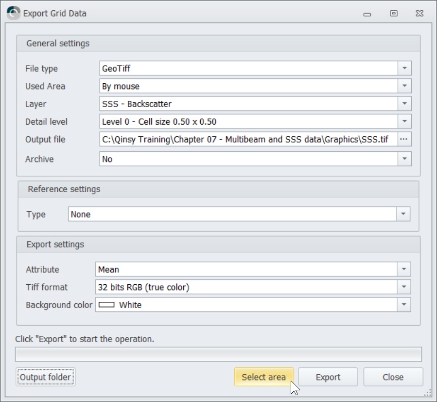
The SSS data can be exported to a Geo TIFF image for further use. Follow the next steps in order to export the data to Geo TIFF:
Select "Export" from the Grid tools tab - Edit option. The following dialog will appear: Export
Set the 'File type' to GeoTiff (*.tif & *.tfw).
Select from which area data will be exported.
Select which type of data will be exported to Geo TIFF by selecting the SSS layer as the Layer to export and set a Detail level.
Change the Output file if necessary. By default this will be in the Graphics folder of the current project.
Set the attribute to Mean depth.
If 'By mouse' was selected, press 'Select area' and define an area to be exported.
Press 'Export' to start exporting the data.
The Geo TIFF images can be used in the Navigation Display or may be useful for third party software programs.
Target Database
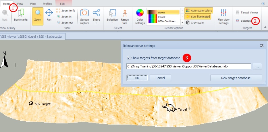
For an overview of the saved targets they can be shown in the Plan View of the Survey Manager:
Go to the Home ribbon tab
Press Settings
Activate the showing of targets and use the browse button [ ... ] to select the target database as created with the Sidescan Viewer.
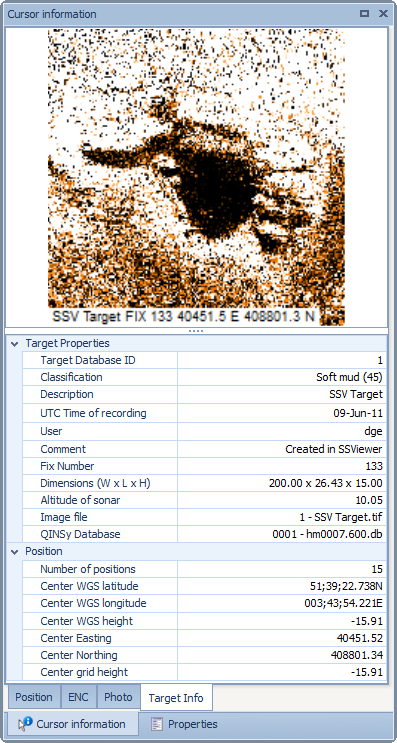
When a target outline is clicked upon, the Cursor Info panel will show all the Target Info as stored in the Target Database:
Target Viewer
In the Target Viewer various databases can be imported, viewed and edited.
In the Survey Manager, Ribbon Tab Home select 'Settings'. Here you can set which database to view. See paragraph Target Database above. The outlines as created in the Sidescan Viewer will be shown in the Survey Manager's Plan View as a visual aid.
Then select 'Target Viewer' to edit the database.
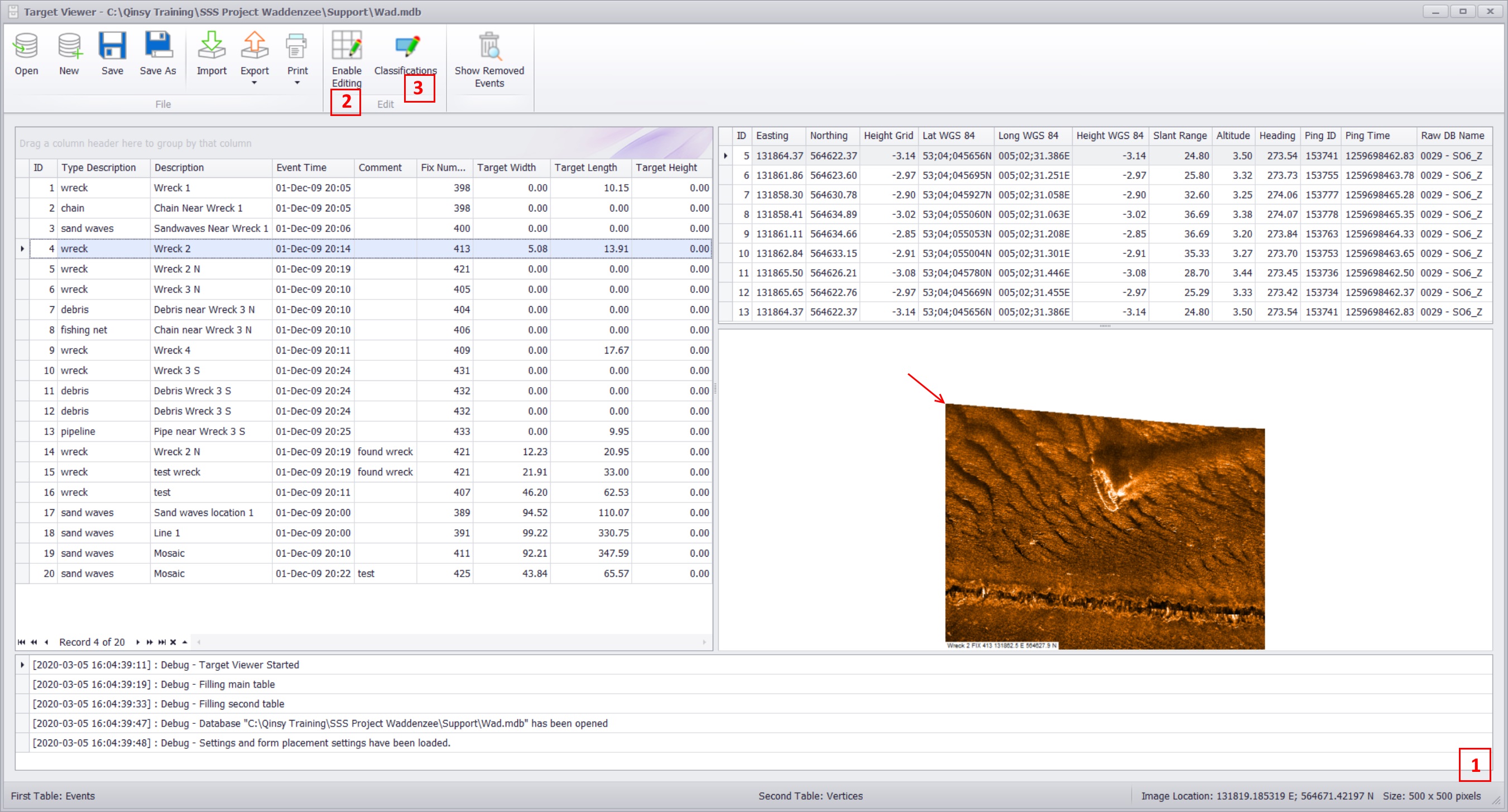
A database looks as follows:
The coordinate shown in the lower right corner of the image panel is the coordinate of the top left corner of the stored image.
Press the option 'Enable Editing' to be able to adjust the Type Description / Description / Comment / Image File or the dimensions of the targets.
Press 'Classifications' to add images to the list of types of targets found in your project.
Info
The Target Viewer has its own F1 inline Help files to explain the functionality of all available buttons and options.
JavaScript errors detected
Please note, these errors can depend on your browser setup.
If this problem persists, please contact our support.