
Fledermaus Tools Menu
The Tools menu contains a number of operations that can be performed on data in the 3D scene.
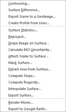
Fledermaus Tools Menu
Contouring
Selecting the Contouring menu option will open the contouring dialog as shown in the Contouring Dialog figure below. It is necessary to specify which elevations will be contoured. The easiest way to generate intervals is to click the Quick Intervals button. Clicking this button will add a number of intervals in the Contour Intervals list box. Contours are generated using predefined intervals based on the range of the input dataset. If a predefined value falls within the bounds of the dataset, it will populate in the Contour Intervals list box. To generate contours at regular intervals specify the minimum starting elevation and the elevation step amount in the Starting Elevation and Elevation Step fields. Once these values are specified, clicking on the Generate Elevation Intervals will automatically add the appropriate elevations to the list. Note that only intervals that fall within the range of the selected data object will be added. Specific intervals can also be added directly by typing the value in the Single Elevation entry field and clicking the Add button. The new interval will then be added to the list. Intervals can be removed by highlighting them and clicking the Delete Selected Values button. The Delete All Values will clear all the entries in the list.

Contouring Dialog
Labels can be generated for the contours by enabling the Label Contours toggle. If the Label Contours toggle is turned on, enter the size of the labels to be generated in the Label Size field. The size entered is approximately the height of the letters in units of the data.
Once the desired contour intervals have been specified, clicking the Apply button generates the contours and makes them appear in the 3D scene. The Cancel button simply closes the dialog without performing the contouring operation.
Note that since 7.6.0, each contour line has an attribute called Elevation with the interval height encoded. This is useful when exporting the contours to Arc, since the contour height can be exported with the data.
Surface Difference
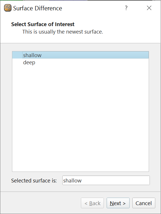
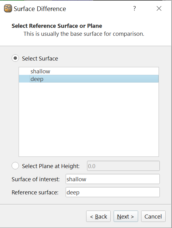
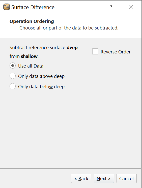
The Surface Difference wizard is used to initiate several kinds of surface-surface and surface-plane queries. Object types that can be queried are selectable through page 1 and page 2 of the wizard, and the type of query to be applied is selected via the query type radio buttons on page 3. The selected query is applied to the specified data objects, and the scope of the query is specified on page 4 of the wizard. By default, the query is applied to the common or intersection area of both input surfaces. However, a polygon can be used to constrain the query scope to within a certain area. A polygon can be loaded from the current polygon selection in the Main Visualization Window by selecting the Use Polygon Selection radial button. Alternately, a polygon can be loaded from an XY text file by selecting the Load Polygon from File radial button.
Page 1
Select the first surface from the list of available surfaces for the difference operation. Click Next to proceed to the next page of the wizard or Cancel to cancel the operation.
Page 2
Select the second surface for the difference operation. Alternatively you can choose to use a plane at a specified height for the second surface. Click Next to proceed to the next page, Back to return to the previous page of the wizard or Cancel to cancel the operation.
Page 3
Select which data to use for the difference operation. Click Next to proceed to the next page, Back to return to the previous page of the wizard or Cancel to cancel the operation.
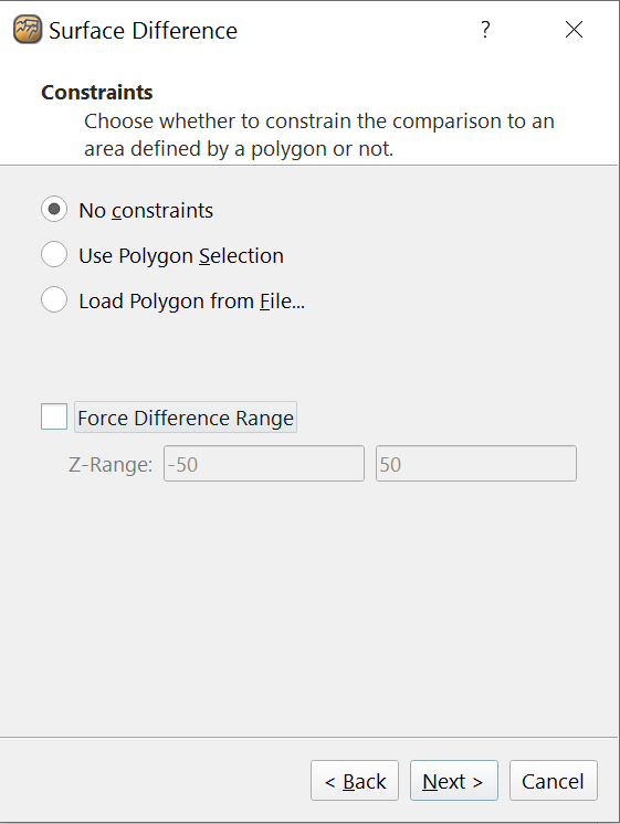
Page 4
Select the constraints of the difference operation. You can optionally specify a Z-Range that you want to force the difference surface to have. The main purpose of this is you want to do multiple surface differences one can optionally guarantee each resulting surface has the same difference range which is particularly useful if one wants to show the difference histogram in the next page to make comparative histogram plots. If one chooses to force the difference range any resulting difference cells outside the specified range will be clipped out. Click Next to proceed to the next page, Back to return to the previous page of the wizard or Cancel to cancel the operation.
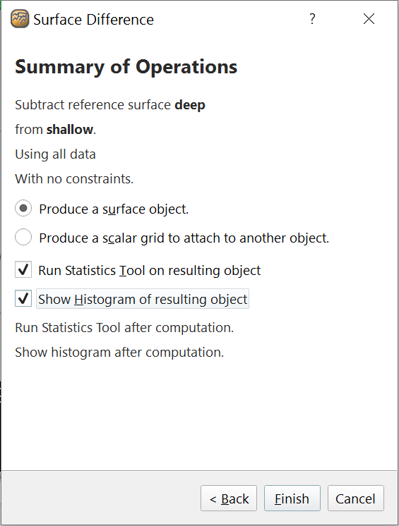
Page 5
Review the selected options for the difference operation. Click Finish to proceed or Cancel cancel the operation. When complete, a Fledermaus static surface will be added to the project representing the results of the surface difference operation. Assuming they are selected one will also see the statistics for the surface difference and/or a resulting histogram of the difference.
Surface Statistics Summary Dialog
This dialog displays the resulting statistical information from the surface difference operation. You can save the statistics to a text file using Save Text As button.
Notes on Surfaces Statistics with Geographic Data
Note that statistics for area and volume as of Fledermaus version 745 will be reported for non-projected data. However, only surfaces in the WGS84 coordinate system are supported. Note that as typical for calculations in geographic coordinate systems, the average latitude is used for calculating the cell sizes. It is assumed that the data is reasonably well distributed. In this case, any loss north of center is made up by excess south. For data sets with more data north or south of the midpoint, the accuracy of the result will vary with latitude and size of the data set. More northerly data sets will have more error depending on how uneven the distribution of the data is. In testing, a comparison of the same geographic data reprojected to UTM was a small fraction of one percent difference in area.
Create Profile(s) From Lines
Clicking this menu option after selecting a line object lets one produce profile objects for one or more lines contained within the selected line object. A dialog box will be shown with the default option to produce one profile object for each line/polyline that the line object contains. Selecting the second option allows one to choose a particular line/poly line within the object to extract as a profile object. As an example if the selected line object contains 3 poly lines you could either choose to extract and create 3 profiles or choose one of 1st, 2nd or 3rd lines to base a profile on.
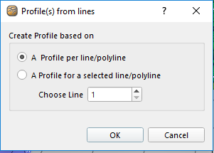
Create Profile from Lines Dialog
Export Scene GeoImage
Export Scene GeoImage Dialog
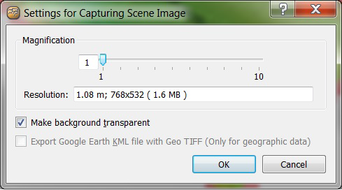
This menu item opens the Export Scene GeoImage Dialog, which is used to create and save a top down, plan view of the current 3D scene as an image. The only export format supported is GeoTIFF.
The magnification can be adjusted to change the resolution and size for the map sheet. The resolution of the image is shown in the box labelled Resolution. The resolution is given in meters, followed by the final output dimensions (i.e. 768 pixels high by 532 pixels wide for this example). Finally followed by the amount of memory used by the image. This last figure may be larger than the size on disk, since compression is usually used to save the image to a file.
Use Make background transparent to convert all white areas in the image to clear, transparent areas. This is useful if the image is to be pasted over non-white backgrounds. If the dataset is geographic, the option Export Google Earth KML file option will be enabled and can be used to export to Google Earth format files. Clicking on the Cancel button will dismiss the dialog and take no action.
Clicking on OK will prompt to save to a file. The only current option is a GeoTIFF. Finally, click Save to finish.
Surface Statistics
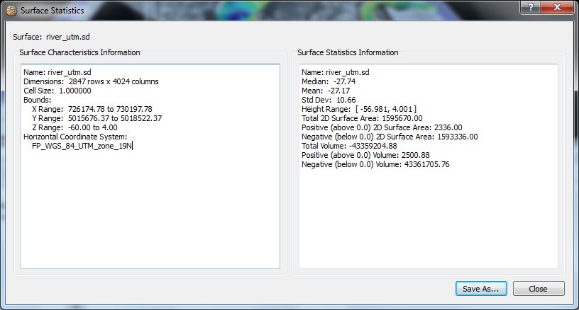
Surface Statistics Dialog
Surface statistics of the loaded surface can be viewed using the Tools > Surface Statistics menu option. Properties of the current data set will be shown in the left text box, while the Surface Statistics Information text box is populated with statistics about the data set.
Notes on Surfaces Statistics with Geographic Data
Note that statistics for area and volume as of Fledermaus version 745 will be reported for non-projected data. However, only surfaces in the WGS84 coordinate system are supported. Note that as typical for calculations in geographic coordinate systems, the average latitude is used for calculating the cell sizes. It is assumed that the data is reasonably well distributed. In this case, any loss north of center is made up by excess south. For data sets with more data north or south of the midpoint, the accuracy of the result will vary with latitude and size of the data set. More northerly data sets will have more error depending on how uneven the distribution of the data is. In testing, a comparison of the same geographic data reprojected to UTM was a small fraction of one percent difference in area.
Reproject
The Reproject tool can be used to convert an SD surface object from one coordinate system to another. The dialog shown below will display both the current (input) coordinate system and the output coordinate system, however only the output coordinate system can be changed.

Reprojection Dialog
Drape Image on Surface
Use the Drape Image on Surface menu option to import an image and drape it over a SonarDTM surface. Click the Browse button to specify the path and name of the image file using the standard file selection dialog, or select from the list of available objects.
When importing an image, the software first cuts out regions from both the image and the DTM that overlap. In order to match areas of the DTM and image, georeferencing must be given for the image in the Georeferencing for image fields. Note that if an image is opened that contains georeferencing (e.g. a geo-tiff), the values will automatically be filled into the fields.

Drape Image Dialog
Next, if the image has a higher resolution than the DTM, the DTM is rescaled to match the image; however, if the DTM has a higher resolution than the image then the image will be rescaled to match the DTM.
Attach Scalar to Surface
Any standalone scalar SD files can be attached to a surface SD file using the Attach Scalar to Surface tool. Once attached, the scalar file can be used to shade the surface and the scalar data will be displayed during any geo-picking operation on the SD surface. The dialog for attaching a scalar is shown in Figure 140.

Attach Scalar Dialog
Mask Surface
Any surface can be masked using the Mask Surface tool. The surface file to be masked will be the currently active data set and it will be displayed in the Apply Mask To text field at the top of the dialog.
The Mask Source can be either an SD object or a supported geo-referenced image file. The Mask Source will knock a hole in the loaded data component files whenever data from the Mask Source is found intersecting any of the loaded data component files. If the Mask Source is a geo-referenced image file, than the Ignore Transparent Pixels checkbox will be activated. This gives the option to either ignore any transparent pixels when masking the surface or not.

Mask Surface Dialog
Extract Area
It is possible to export a region of the currently selected surface by selecting Extract Area from the Tools menu. This menu option brings up the Bounds Entry dialog box, where a rectangular sub-region of the surface may be extracted from the currently selected surface or scalar object (see image below).
A region to cut may be specified in one of three ways:
- Custom Min and Max: specify a rectangular sub-section of the data by giving the lower left and upper right coordinates of the box
- Center and Radius: specify a rectangular sub-section of the data by giving the center point, x radius, and y radius of the box
- Corner and Size: specify a rectangular sub-section of the data by giving the lower left corner plus the width and height

Extract Area Dialog
Calculate Slope
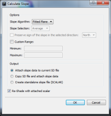
Calculate Slope Dialog
Surface slopes can be calculated using the Tools > Compute Slope menu option. The dialog box in the figure above allows the user to compute a surface that represents the maximum slope at each grid center of the currently selected SD. The generated surface will have the same dimensions as the original surface file and represents the maximum slope from each cell to any of its neighbouring cells.
For the generated surface, each cell represents the maximum slope to any of its neighbours written in decimal degrees. You can optionally specify the slope range bounds for the generated surface. This is useful if you want the range to correspond to a particular range of colors in a given color map.
The created scalar file can then be used in the shading process to drape the scalar color over the DTM. The values of the scalar can also be attached to the original surface. This means that when the surface of the object is picked in Fledermaus it will return X, Y, Z, and slope. Alternatively the user may create another surface where the Z value of the DTM is the slope.
If the resulting surface will be an attached Scalar to the current SD or a copy of the current SD, the SD can be re-shaded using the new attached scalar if Re-Shade with attached scalar is toggled on.
Calculate Rugosity
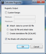
Calculate Rugosity Dialog
Rugosity is a measure of surface roughness and it can be created using the Calculate Rugosity command. The Gridding Window specifies the grid size surrounding a cell that will be used to calculate the rugosity value. By default the output surface will contain the full range of rugosity values, however a custom range can be specified to restrict the output to the user supplied values. There are three output options for the generated surface, with the default being to attach it to the original source SD file. There is also an option to create a copy of the source SD before attaching the rugosity, as well as an option to create a standalone SCALAR file.
If the resulting surface will be an attached Scalar to the current SD or a copy of the current SD, the SD can be re-shaded using the new attached scalar if Re-Shade with attached scalar is toggled one.
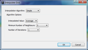
Interpolate
The surface interpolation tool allows for small holes in a surface or scalar to be filled in using values from one or more of the surrounding cells. The interface for setting up the interpolation is displayed in the figure below. Four options are available for determining the interpolated values:
Average: Calculates the average value of all surrounding cells
Minimum Value: Uses the maximum of all surrounding cells
Maximum Value: Uses the minimum of all surrounding cells
Fixed Value: Uses the value supplied by the user
Interpolate Dialog
Once the interpolation method has been chosen, the next step is to determine what cells will be filled in by the interpolator. This is done by setting the minimum number of neighbours required for a cell to be filled in, ranging from 1 to 8. You can also set the number of times the algorithm runs over the entire grid by setting the Number of Iterations pull down menu.
Export
It is possible to export a surface grid from Fledermaus by clicking the Export Surface menu option. The following figure illustrates the Export Surface dialog box that includes several options to tailor how the surface will be exported. These include:
- ASCII Z
- ASCII XYZ,
- ArcView ASCII Grid,
- Raw binary grid
- NetCDF/GMT Grid
- Export GMT Grid
- Floating Point GeoTIFF Grid
- QPS GRD3 (Medium Layer Only)
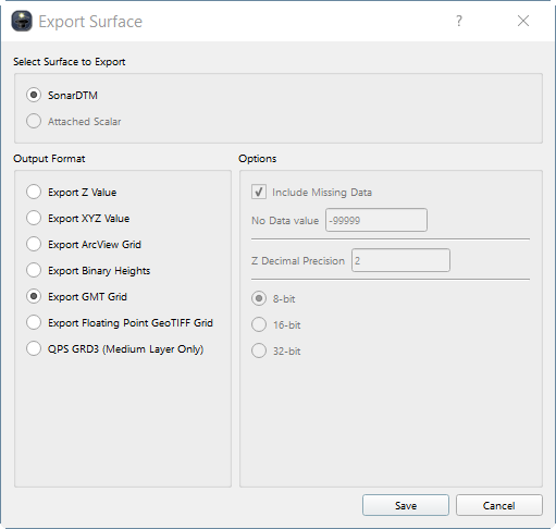
Fledermaus Export Dialog
Exported Surface can either be a SonarDTM or an Attched Scalar depending on what you choose from Select Surface to Export.
When saving the data, areas of the surface containing no data may be included with the output file if the Include Missing Data option is on. If missing data is included, a special value is written for these data points, indicated by the No Data Value text field.
When writing a binary file, you may specify either writing an 8-bit or 16-bit, or a 32-bit unsigned integer values representing the heights.
When exporting to ASCII X and XYZ Grids, there is an option to specify decimal precision of the Z value being written.
Render Movie
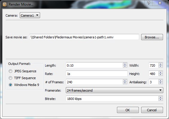
Render Movie Dialog
The Fledermaus package contains tools that support the creation of standalone digital videos from flight paths produced within the visualization system. These videos can be viewed by most computer video players (such as QuickTime or Windows Media Player) and display the data at its full resolution, not the reduced "exploring mode" resolution used when animating in Fledermaus.
Camera: This section allows you to specify which camera view you would like to render.
Save movie as: This will determine the root name for all movie frames that are generated.
In the Output Format field, you must select the file format to save the images as---TIFF or JPEG. JPEG images are slightly lower quality than TIFFs but use considerably less hard disk space. Your saved file will have a four-digit number and a file extension added to it. If, for example, your movie contains 300 frames, you select JPEG as the image format and "D:\Fledermaus Movies\camera-path.jpg" as the base file name, the files generated will be stored in D:\Fledermaus Movies\ and named camera-path.0001.jpg, camera-path.0002.jpg, camera-path.0003.jpg, . . . camera-path.0300.jpg.
The final option in the Render Movie dialog is Antialiasing, Antialiasing works by rendering each frame at a higher resolution and then scaling them down to the resolution of the output movie. This results in a higher quality image but causes rendering to take quite a bit longer. The antialiasing factor is the size difference between the rendered frame and the output movie---an antialiasing factor of three will mean that the render window will by three times as wide and high as the final movie.
In order for rendering to work properly the entire Render Window must be visible on the screen with no other windows in front of it. (The exception to this is on Macintosh computers; on these machines rendering will still work properly even if other windows are in front of the Render Window.) Since the render window will be as big as the output movie frames (larger if antialiasing is used), it may not always be possible to render an entire frame at one time.
After you have adjusted all the parameters, position the Render Window so that the entire window fits on the screen and is not covered up by any other windows. Don't worry about the Data Sets window or Render Movie dialog as these will both disappear once rendering starts. You must also ensure that there is no screen saver active on your machine since it would obscure the Render Window when it activates. Please see your operating system manual or IT support personnel for instructions on disabling your screen saver if you don't know how. Once you are ready to proceed, click the OK button to begin rendering. Rendering will probably take several minutes to complete, during which time the Render Window must remain unobstructed.