
3. Qinsy Online
In the previous chapter the interface settings of the sensors in the database with their offset positions relative to the object reference point were described.
Also, the geodetic settings were entered.
The next step is to go Online 
The Online part of the software is what is used to record the data during the survey.
On this page:
Controller
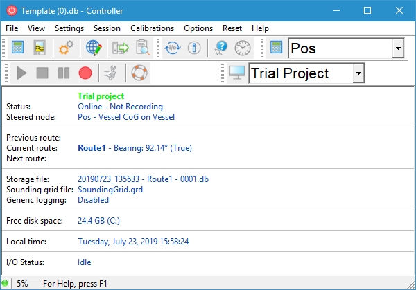
The ‘Controller’ is the first dialog which appears when going online. This dialog will manage and control the Online session.
Computation Setup
With a new database, a number of settings need to be entered so that the position and depth are calculated correctly. This is done in the “Computation Setup wizard”.
Clicking on the
Computations are needed by Qinsy to link e.g. the depth readings from the echosounder to the position readings of the antenna.
Whenever a new template is started, one computation is created with default settings. This computation needs to be checked to see if the settings are usable for this kind of survey.
It is also possible to create a second, third, nth computation. When multiple position systems are available, multiple computations can be created, each computation using one position system.
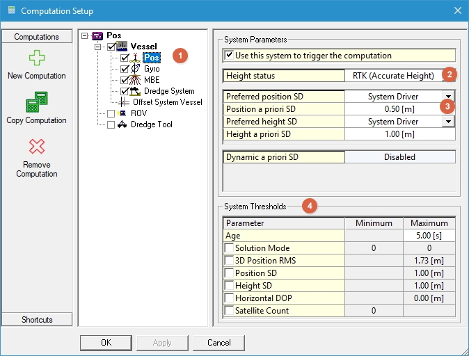
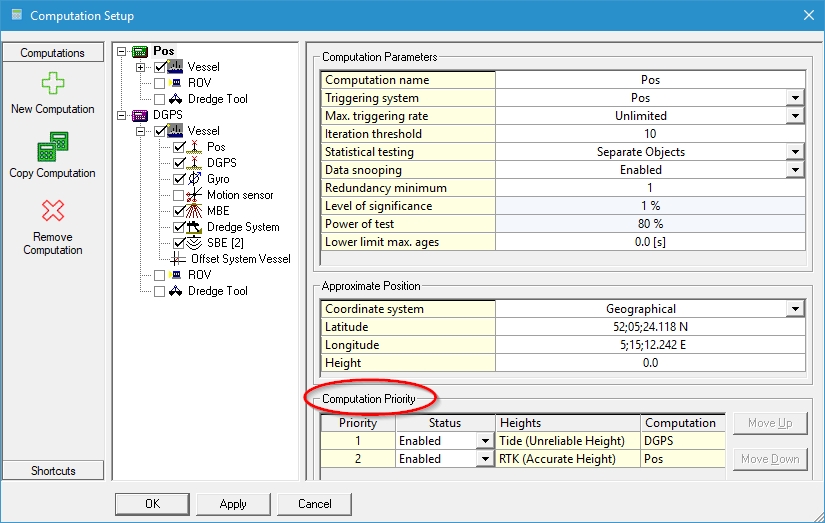
- Select the Position system.
- Select the Height mode of the positioning system. For RTK DGPS systems the height status should normally be set to Accurate.
This means that the Z of the position system is used to calculate the depths.
Otherwise, select Unreliable. This means that tidal levels and the Mean Sea Level model will be used to correct the depths. - Set the a-priori SD correctly (for more information see the 'How-to Total Propagated Error' in the Knowledge Base).
- Enter positioning System Thresholds. If one of the thresholds is exceeded, the computation will fail and Qinsy will automatically switch to the secondary computation (if available).
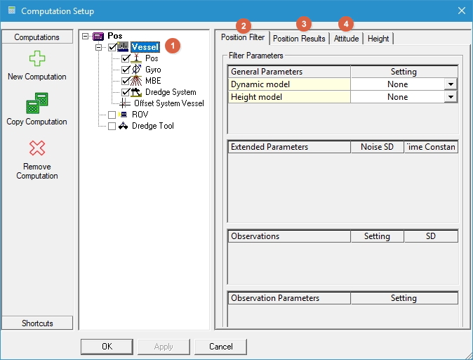
- Select the Vessel.
The position of the object is by default taken directly from a positioning system or surface navigation system. This page allows for using a Kalman Filter in order to smooth the raw positions from the computations. Optionally input of heading, height, and/or speed sensors can be integrated into the Kalman Filter.
The Position Results page is for setting how the object node positions (including echosounder transducer positions) are interpolated and predicted following the position updates or Kalman Filter updates at a triggering system update time.
When more than one gyro or motion sensor is available, select which system is to be used as primary system.
More about Kalman Filtering
See for more information about Kalman filtering the 'How-to Smooth Vessel or ROV Track' in the Knowledge Base.
Height Settings
In order to relate the measured depths to the vertical datum used for the survey, it is necessary to know the height of the transducer with respect to this datum.
If a positioning system is used that outputs an unreliable height (e.g. DGPS), then a number of parameters need to be set in the Controller.
These settings are not needed for a system that outputs an accurate height (e.g. RTK DGPS).
More information on Height settings can be found in the 'How-to Height' in the Knowledge Base.
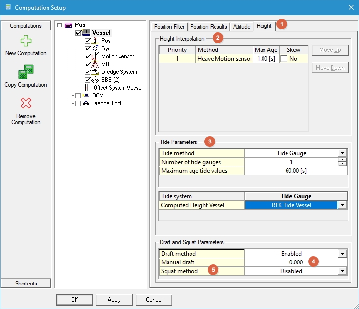
- Select the Height tab.
- Select the heave method that will be used to correct the height data.
- Set the tide method and the tide gauges / files that need to be used for the depth correction (see for more information the 'How-to Apply Tide' in the Knowledge Base).
- Enter the draft of the vessel. This is the draft relative to the draft reference as entered in the template setup.
- If a squat model was defined in the template setup, enter the squat method and the related parameters.
If the primary computation is not working correctly, Qinsy will automatically switch to the secondary system.
Echosounder Settings
Under certain circumstances data from an echosounder can contain a lot of noise. Although noise should preferably be removed using filters on the echosounder itself, this is not always possible.
In order to clean the data Qinsy offers a number of online filters that can reject most of the larger spikes in the data.
Use the table under 'Exclude Data When' to set various filters, plus the tab Quick Blocking.
Open the Echosounder Settings window from the Controller
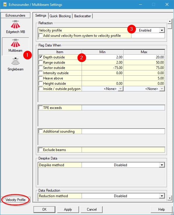
- Select the echosounder; singlebeam and multibeam have different options
- Enter values for filtering
- Enable the velocity profile (if used).
Use the F1 inline help function for information about the different filters.
Filters affect data in Sounding Grid and DTM file only
The echosounder filters only affect the data that is stored in the Sounding grid or in the DTM file.
All depths will be stored in the database as raw depths.
Sound velocity profile
The sound velocity is needed to correct the depth readings from the echosounder to true depths, depending on the echosounder settings.
Most echosounders allow the input of a single sound velocity, whereas Qinsy is able to use the entire sound velocity profile as measured.
To enter a sound velocity profile, select the Velocity Profile group to make the velocity profile dialog visible.
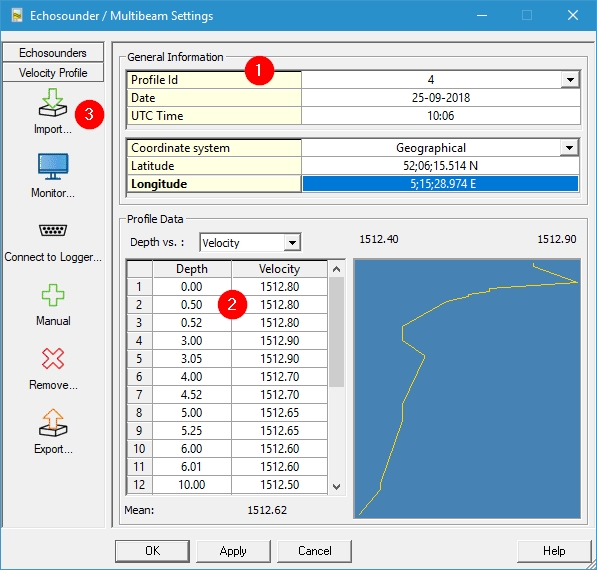
- Several profiles can be defined in the database; each gets its own Profile Id.
The profile location and time are administrative only and are not used for the correction. - The profile can either be entered manually by adding observations (depth / velocity)
- Or the profile can be imported as a text file generated by a sound velocity probe.
Session Setup
Before starting the survey a number of settings need to be entered in the Session Setup. These settings include line planning, storage and fixing options.
In the Controller click on the Session Setup 
Planning
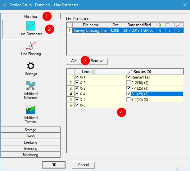
- Select the “Planning” group to enter the line planning.
- Select the “Line Databases” button.
- Use the Add button to add a previously defined line database file. (Use the Line Planning option for this.)
- Enable/disable lines from the line database file.
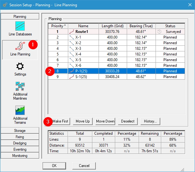
- Select the “Line Planning” button.
- Select one of the lines.
- The line at the top of the list is selected as the first line to be sailed. Use the button “Make First” to put a line at the top of the list.
Use the "Move Up” and “Move Down” buttons to move the lines in the list.
Using the “Page Up" and “Page Down” buttons
During the survey the next / previous line from the line planning can be selected using the “Page Up" and “Page Down” buttons on the keyboard.
Storage
Database
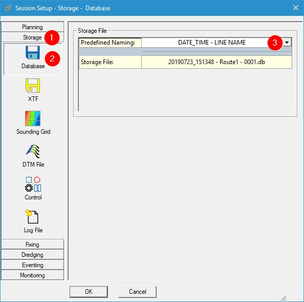
- Select the “Storage” group in the Session Setup to make the storage settings visible.
- Select the “Database” button.
- Select one of the predefined file types or use a User Defined filename. If a prefix is used, then each database will get a sequence number.
Whenever a new recording session is started the sequence number will be increased by one.
Automatic and manual recording
When recording is started, databases are always recorded.
DTM files (e.g. QPD's) and grid files are optional and should be enabled manually.
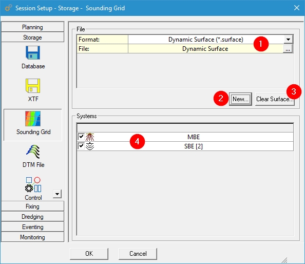
Sounding Grid
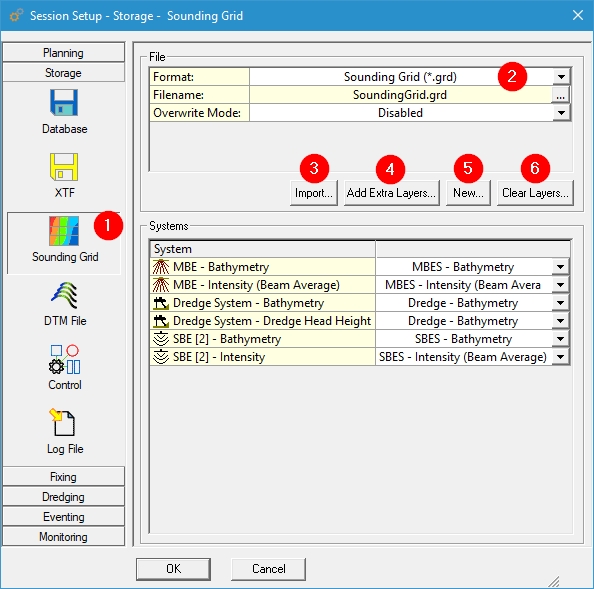
- Select “Sounding Grid” to enter the storage properties for the Sounding Grid.
- Enable storage to a Sounding Grid.
- Importing an existing file can be done.
- You may add extra layers to the selected grid.
- Or select New to create a new Sounding Grid/Dynamic Surface.
- You may also clear layers within the grid.
- Each system can store its data to its own layer in the Sounding Grid; select a specific layer from the pull-down menu for each system.
Create a new Sounding Grid
A sounding grid is a rectangular raster that is composed of a number of cells.
Each cell has a coordinate and will store a number of parameters like:
- Mean depth - This depth is based upon all the soundings that lie within that cell
- Deepest point - The deepest sounding lying within that cell.
- Shallowest point - The least depth sounding lying within that cell.
- Standard deviation - The spreading of the soundings used to generate the mean depth.
- Hit count - The number of soundings used to generate the mean depth and standard deviation.
The grid format does not have a boundary and is created on-the-fly.
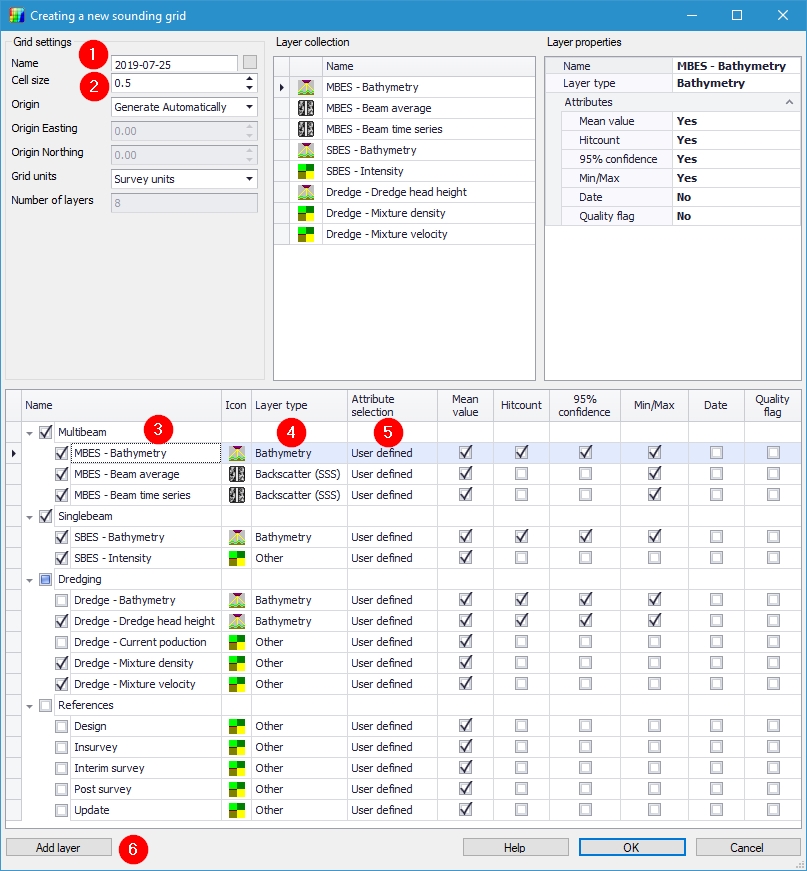
- Specify the file name.
- Enter the base cell size.
- Select the systems which will be stored in the Sounding Grid.
- Edit the Layer type if necessary.
- Select the attributes which should be stored in each layer.
- Add a layer if necessary.
Create a new Dynamic Surface
A dynamic surface is a grid file which is filled while recording data.
- Enable storage to a Dynamic Surface.
- Select New to create a new Dynamic Surface.
- You may also clear the complete surface.
- Select the system(s) used for recording the data.
After pressing "New" the following dialog will open:
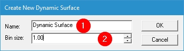
- Change the Name if necessary.
- Adjust the Cell Size if necessary. For dense data a small size can be set (0.25 or 0.5 meters).
For widely spaced data a large size can be set (deep water e.g. 50 meters).
By pressing OK, the Dynamic Surface is created and will be filled when you start recording.
Info
Whereas with a Sounding Grid you can choose not to create *.qpd's, while sailing with a Dynamic Surface *.qpd's will automatically be created.
DTM file
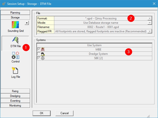
- Select “DTM File” to enter the storage properties of DTM data.
- Select the output format for the storage of the corrected data. The most commonly used format is the Qinsy Processing format.
- Choose the system(s) of which data needs to be stored.
Reduced and Normal processing format
There are two types of Qinsy Processing format: reduced and normal.
The difference lies in the fact that the reduced format doesn't contain data that did not pass the online filters while the normal format stores all data points.
The datapoints that didn't pass the online filters will be flagged.
Control
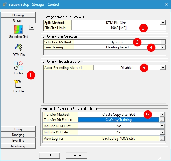
- Choose the "Control" option from the Storage group for further settings on logging data.
When collecting large amounts of data (e.g. multibeam) the resulting database can grow to a respectable size when sailing longer lines.
Split the databases to a size that can be handled by the processing software using a number of splitting options.It's possible to select lines automatically, choose from:
- Disabled (select manually)
- Planning: the next line is the one down the list in the Planning group.
- Dynamic: the line closest to the vessel is automatically selected.
Line bearing selection method has the following options:
- Planning: the bearing selected in the Planning Group is used.
- Heading based: line has the direction of the forward heading of the vessel. When vessel turns, the line is reversed.
- Closest distance to SOL or EOL: line is directed so that more than half the line is ahead. When vessel is halfway along the line, it reverses (when not logging).
- Qinsy has the option to automatically start and stop recording (see for more information the F1 inline help of this dialog).
- Recorded data can automatically be copied or transferred to another location on the computer or network after finishing a survey line.
Select to copy or to move the DB files. Select the folder (can be across a network).
Fixing
Fixes are used e.g. for displaying depths in the navigation display, but are also stored in the database.
Before Fixing can be used, a number of parameters need to be set.
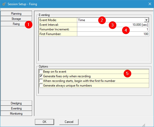
- Select the “Fixing” group in the Session Setup to enter the fix settings.
- Select the fix (event) mode (see the F1 inline help of this dialog for more information).
- Enter the fix interval in meters or seconds.
- Set the fix number increment and the first fix number.
- Use the check boxes to set additional parameters.
Recording
The Controller is used during the Online and Replay sessions to coordinate the flow of data.
During the online session the recording of data and the line selection is done using the Controller.
There are 4 operational modes for the Controller, of which 2 relate to both the online and the offline session.
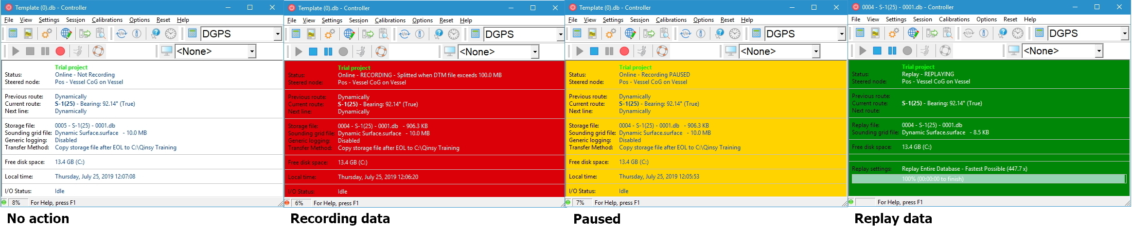
The data flow is controlled by the icons in the tool bar or by using the function keys on the keyboard:


Whenever recording is stopped and started again and the sequence numbering is active, a new database will be created starting with the next sequence number.
Creating displays
Qinsy Survey has the option to create any number of pre-defined displays. A number of display types can be selected.
Each display can be customized and can be given a location. A defined display belongs to a display set. Each Qinsy user can create their own set of displays.
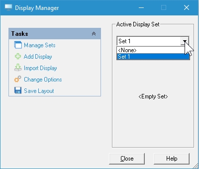
Select the Display Manager icon 
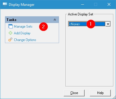
- A Display Set must be selected, by clicking on the down arrow
- When there is no set available, select “Manage Sets”
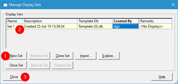
- Create a set with the “New Set” button.
- Enter a name for the set.
- To add displays to the set, close this window and return to the Display Manager.
Use the “down arrow” to set the created display set as the “Active Display Set”.
Select "Add Display" and the following dialog appers:
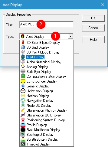
- Select the desired display.
- Give it a descriptive name.
Repeat this for all the displays needed during this project.
Too many displays
Be aware that some system drivers automatically start their own displays.
It might therefore be most efficient to first define all the systems in Database Setup, start the Console and check which displays are already available.
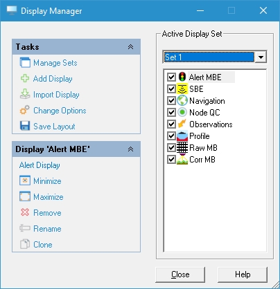
Tick the box of a display to display it.
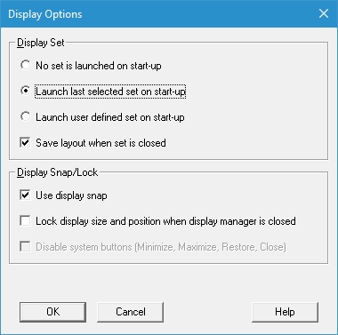
The displays can be saved each time the Controller is closed, and retrieved every time the Controller is started.
Select “Change Options” and tick the desired options:
More space on screen
Many displays have the option to turn off the status bar, tool bar and menu and title. Turning these off will create more space for additional displays as well as creating a less cluttered display.
Select “View” from the respective menu bars and deselect the appropriate options. Double clicking on the display will bring back the menu bar and title.
Visible at all times
Use the option “Always on top” from the “View” menu to make sure that a window stays visible at all times.
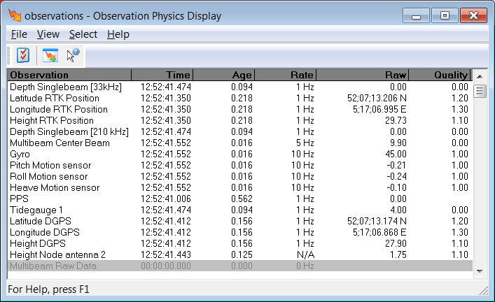
Observation Physics Display
The Observation Physics Display shows the raw data coming from external sensors which is very useful to check whether the correct drivers heve been selected in the Database Setup.
The data is decoded by the driver selected in the template (Database Setup). Default corrections and velocities are applied where required.
Add an Observation Physics display in the Display Manager:
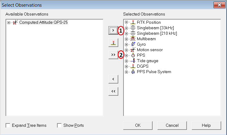
- Select the observations to show in the display and use the > key to select them.
- Or use the >> key, to select all available observations at once.
Add extra columns
Use 'Properties' from the View menu to add extra columns.
Use the inline F1 Help for more information about the Observation Physics Display.
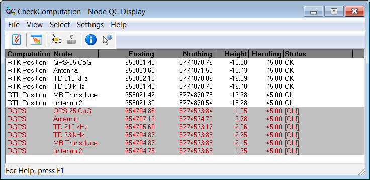
Node QC Display
Useful display to check whether your computation is working properly and whether all nodes are computed as required.
Node position calculation
A node is a position on an object, relative to the object's coordinate frame. For each computation cycle, the node's position is calculated.
If multiple computations exist (multiple GPS receivers in use) the node is calculated separately for each computation.
The Node QC display shows the calculated position and the status. If the status is good, the background remains white.
If the status is BAD, the background turns gray and the node in question is displayed in red.
Add an Node QC display in the Display Manager:
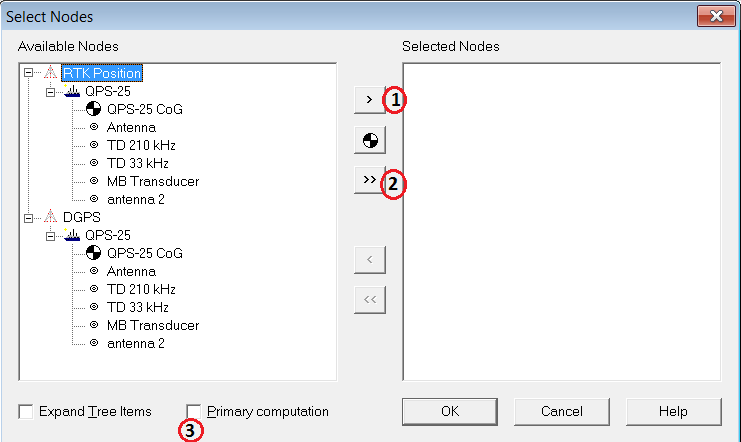
- Select from the available nodes, the nodes to show in the display and use the > key to select them.
- Or use the >> key, to select all available nodes at once.
- Disable Primary computations, to make all available computations visible.
See for more information and extra options of the Node QC Display the F1 inline Help.
Navigation Display
The Navigation Display is used to display a top view of the area with background charts, the sounding grid and the vessel (track).
Add a Navigation display in the Display Manager.
Below is an example of a Navigation display with ENC background, line database file and sounding grid.
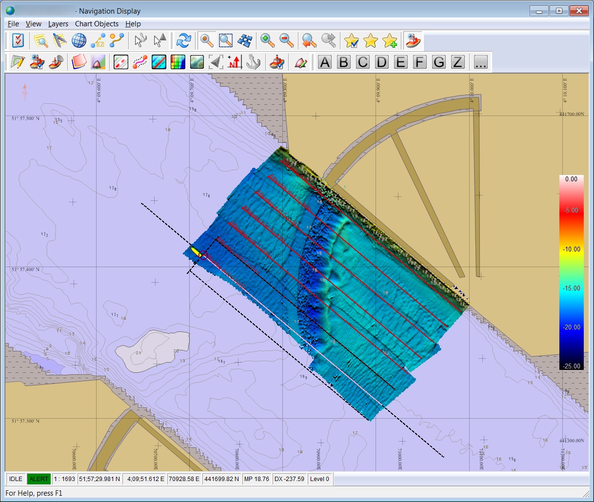
See for more information and all options of the Navigation Display the F1 inline Help.
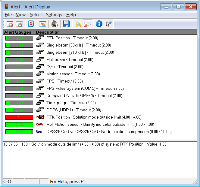
Alert Display
The alert display was developed to warn the user about failing I/O of interfaced systems.
Also options for received or calculated values that do not meet criteria set by the user can be entered here.
Add an Alert display in the Display Manager:
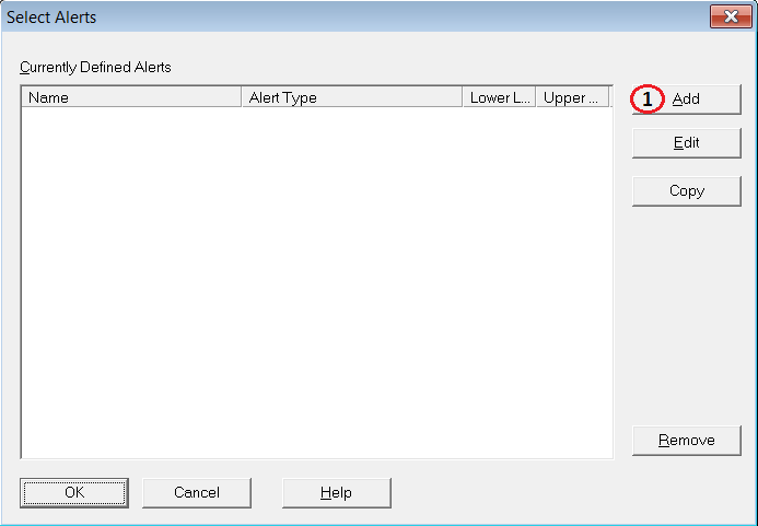
- Select the Add button
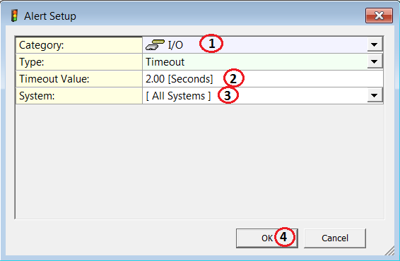
- Select I/O as category
- Enter a Timeout value
- Select a System (or All Systems)
- Click on OK
In the example above an alert will be fired when a system doesn't give an output to Qinsy for more than 2 seconds.
Other examples of alerts:
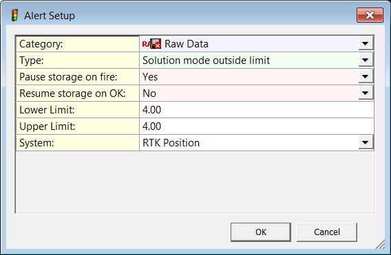
An alert will be fired when the solution mode of the position system is not 4 and when the alert is fired during recording the recording will stop automatically.
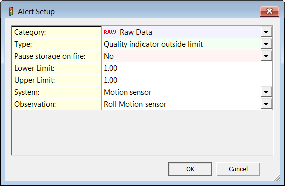
An alert will be fired when the quality figure of the Roll is not 1.
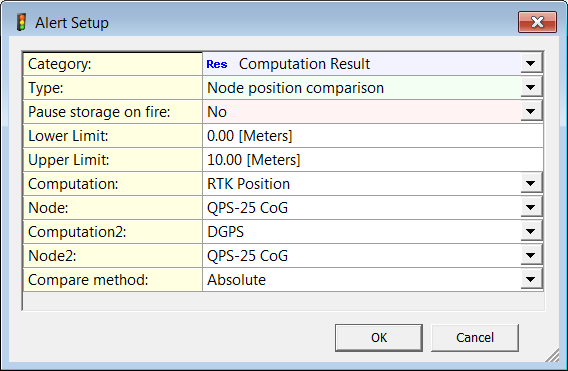
An alert will be fired when the difference between the CoG node calculated with computation RTK position and calculated with the compuation DGPS is more than 10 meters.
Info
There are many more alerts. Scroll through all the available alerts and decide which ones can be useful for your operation.
All available displays
| Display Type | |
|---|---|
| 3D Error Ellipse Display | Show the error ellipse of the GPS antenna position. |
| 3D Grid Display | Make use of the sounding grid to show a 3D image of the seafloor including a 3D image of the survey vessel and other objects when available. |
| 3D Point Cloud Display | Use this display to show Multibeam point data in 3D. |
| Alert Display | Show alerts on I/O, quality indicators and values. |
| Alpha Numerical Display | Show all kinds of available information in numerical form. |
| Analog Display | Show various information such as pitch, roll, heading in an analog view. |
| Bulls Eye Display | Helpful when navigation to a certain point is required. |
| Computation Status Display | Show the status of a selected computation, including the results of all kinds of quality tests. |
| Echosounder Display | Show raw echosounder data in a graphical view. |
| Generic Display | Visualize all kinds of available information in a numerical form. |
| Gun QC Display | Show status of the air guns. |
| Helmsman Display | This display includes a left / right indicator, distance in line indicator and a track view. |
| Horizon Display | Show the movement of the vessel relative to the horizon. |
| Navigation Display | A multi-functional display which shows the vessel, line planning, sounding grid file, ENC's and much more. |
| Node QC Display | Useful display to check if your computation is working properly and if all nodes are computed as required. |
| Observation Physics Display | Show all raw observations coming in in a numerical view. |
| Observation QC Display | Show the quality of raw observations (mainly used for raw GPS data). |
| Positioning System Display | All available information is visible here for each positioning system such as positions, used satellites, RWS values, DOP values etc. |
| Profile Display | A realtime profile is shown of the vessel, the seafloor and depth measurements such as from echosounders. |
| Raw Multibeam Display | Show raw data of a multibeam sensor. |
| Scatterplot Display | Create a scatterplot to show the differences between two nodes. |
| Sidescan Image Display | Show a sidescan image. |
| Skyplot Display | A plot of the sky is shown with all available satellites. |
| Swath System Display | Show corrected multibeam data including blocking parameters and TPU error ellipse. |
| Timeplot Display | Time series of all available data. |
| ADCP Display | The strength of the current and the bearing of the current throughout the water column around the vessel can be viewed in this display. Only available when an Acoustic Doppler Current Profiler system is available in Database Setup. |
| Sub Bottom Display | Use this display to view the raw data while recording it with a Sub Bottom Profiler. Only available when a Sub Bottom Profiler system is available in Database Setup. |