Qimera Time Series Multiplot Dock

Qimera - Time Series Multiplot

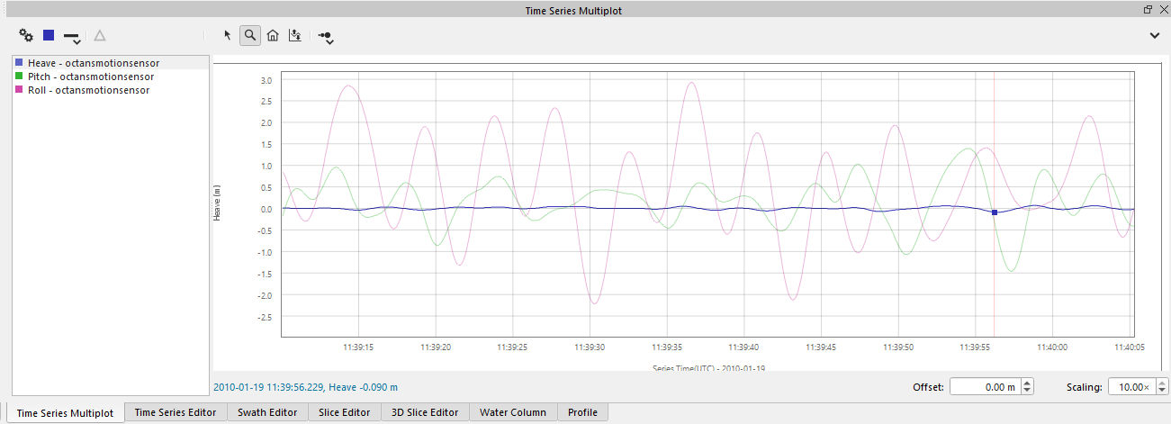
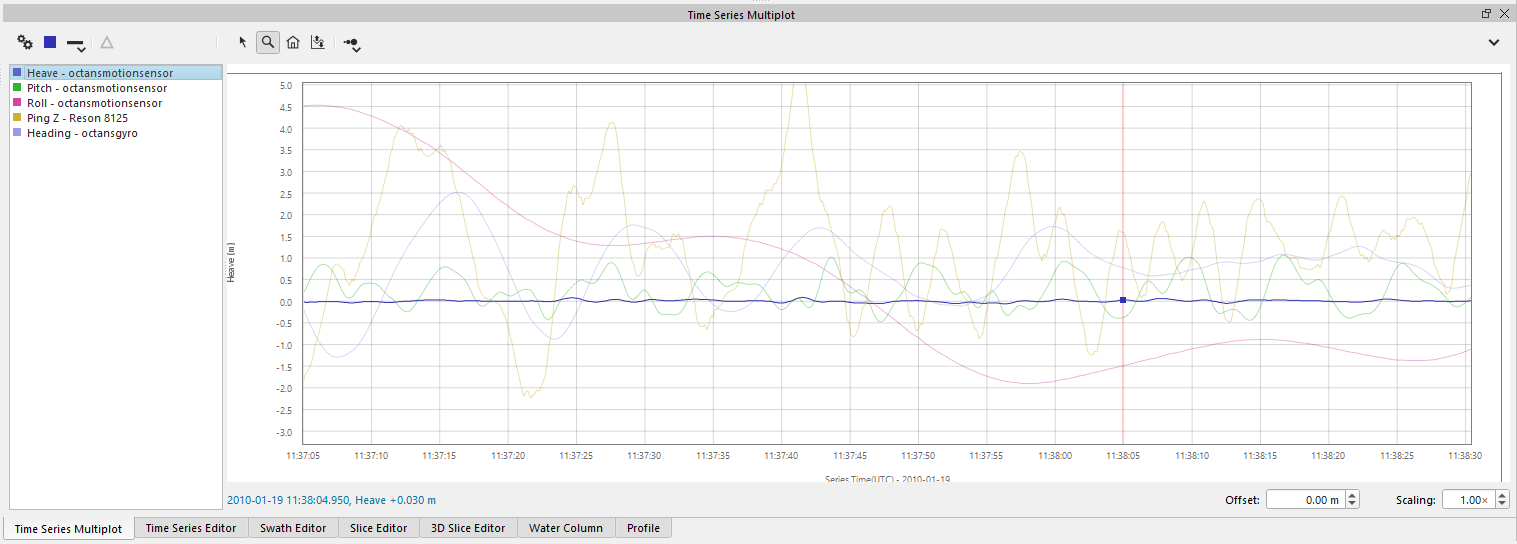
The Time Series Multiplot allows for temporal visualization of attributes with different scales and units on the same piece of virtual 'paper'. It allows you to correlate time series information from the currently selected file in your project. You can easily move selected time series attributes up or down on the paper and/or change their vertical scale. The configured attributes appear in a list view on the left side of the window. The plotting area displays the attributes by color and line pattern. The horizontal axis of the plot is time. The vertical axis changes according to the currently selected attribute to conserve screen space except during image export. The cursor label in the lower left of the plot area displays the time and value of the selected attributes. The Offset and Scaling spin-boxes display the vertical offset and vertical scale of the currently selected attribute(s). The Multiplot can display data that was extracted during the initial import of the source file, as well as data that is computed during the refraction process. The Multiplot additionally allows for creation of a simple mathematical difference series that can be added to the display.

For information on plot grid navigation and editing, see the page in the manual on Qimera Plotting Grids. If your plot ever gets a bit foobar, simply select all series' in the list view and set the Offset to zero and the Scaling to 1.0.

Configure Series

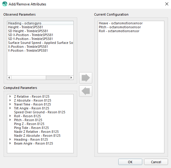
This will launch the Add/Remove Attributes dialog shown below. Use this to configure what gets displayed on the Multiplot grid. If you change the line selection, the Multiplot will try to utilize the same configuration for the new line, if possible. Missing attributes will be discarded. Use the arrow keys to add or remove time series information from the Multiplot configuration. On the left of the dialog are lists of the observed and computed parameters. Observed parameters are those that were extracted from your raw sonar data and potentially used during processing. The computed parameters are the attributes that are contained in the QPD file after processing, see examples below. As you select and move items into or out of the configuration, they will also move visually between the various lists. The beam computed parameters can be found as sub-lists of the root attribute, such as 'Travel Time'. Click OK to complete your configuration or Cancel to return to the current configuration.

Example of computed parameter: Ping Z

The depth of the transducer below datum. If the Vertical Referencing is set to ‘None' this will be the depth of the transducer below the water line calculated with Depth / Pressure, Heave, Draft / HADR / Transducer Z value and any Static Shift. If the Vertical Referencing is set to RTK, this value is just a positioning system interpolated with heave if available, plus any vessel offsets. Finally, if Vertical Referencing is set to Tide, the calculation will be equivalent to 'None’ plus a tide value.

Color Button

This button will change the color of the currently selected attributes.

Line Pattern Button

This button will change the line pattern of the currently selected attributes. If you click and hold the button, you will see a drop down list of the choices. If you simply click, it will cycle to the next line pattern. The choices include: dots, dashed line, dot-dash line, dot-dot-dash line, and solid line. Some line types are shown below.

Delta Button

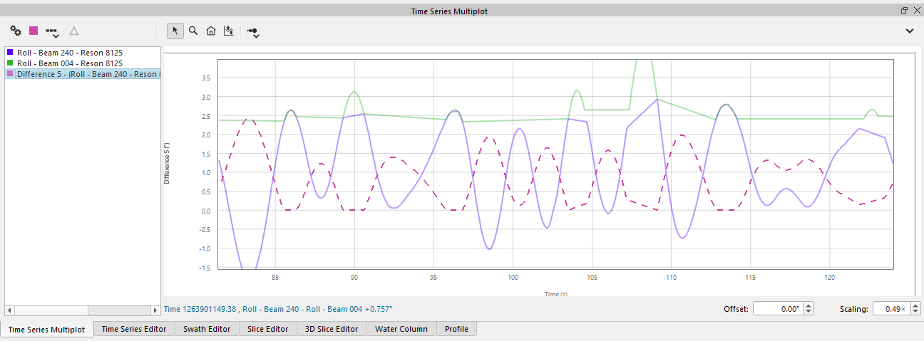
This button will compute the difference between 2 attributes with the same units and add the series to the plot. Simply select 2 attributes with the same units and click the button. Below is a difference plot of Beam 240 Roll minus Beam 004 Roll. The order of the difference (a - b) is based on the selection order of the attributes. The series attribute name and the tool tip of the button will also indicate the order.

Zoom Out Button

If you have zoomed into an area of the plot, this button will zoom out to the extents of the currently viewed attributes. All attributes share the same time axis.

Explore Mode

This is the primary exploration mode of the tool. As you move your cursor over the plot, the label in the lower left of the window will update to show the current time and value of the selected attributes. If you have loaded a Route Layer a KP value will be displayed. A tracking ball will follow the location in time along the currently selected track in the 4D View. If you click/drag the plot grid, you can pan around the data. If you hold Ctrl and click/drag, you can move the currently selected attributes up or down on the plot grid. As you do this you will notice that the Offset spin box changes to show what the current vertical offset is from the original state of the plot. You can additional use the spin box to control the offset of the currently selected attributes. If you use the mouse wheel at the same time as holding down the Ctrl key, you can change the vertical scaling of the currently selected attributes as described by the explicit Scaling Series Mode below. Shifting or scaling the currently selected series works in all modes using the Ctrl key to modify a click-drag or mouse wheel action. Holding the Shift key during click-drag will allow panning in any of the modes. The mouse-wheel will zoom in/out of the plot.

Zoom Mode

When in zoom mode, simply click and drag an area of the plot to zoom the time window. Multiplot only allows for zooming along the time axis. To return to the original plot, simply click the Zoom Out button.

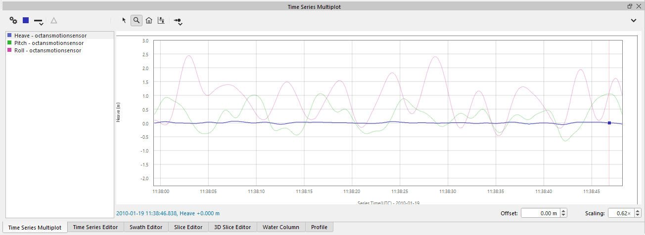
Multiplot Before Zoom

Multiplot After Zoom

Scaling Series Mode

This will allow you to change the vertical scale of the selected attributes. As you click/drag the cursor left/right or up/down, the vertical scale of the selected attributes will increase or decrease. You can also see the change in the Scaling spin box in the lower right corner of the Multiplot window. When attributes are added to the Multiplot, the initial vertical range is Rmin - Rdelta to Rmax + Rdelta where Rdelta is Rmax-Rmin.

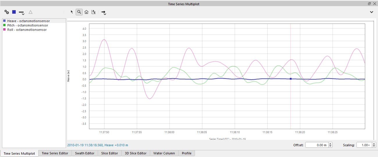
Roll Before Scaling

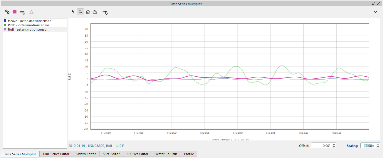
Roll After Scaling

Point Size

This button will allow you to change the size of the plotted points and lines. Sizes range from Small to XX-Large. Clicking on the button will cycle to the next size. Click and hold to get a drop down menu of sizes to choose from.

Time Series Multiplot Menu

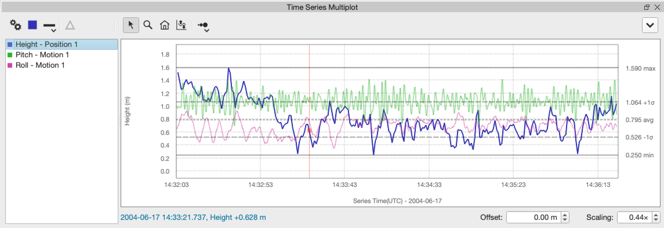
Show Statistics

This setting turns on the statistics view for the currently selection time series. It will show the minimum and maximum as solid lines, the +/- 1-Sigma as dashed lines and the average as a dotted line. Value labels will appear on the right side of the tool.

Show Height at COG

This setting only affects the display of the Height attribute. When enabled the Height plot will be transformed to the (0.0, 0.0, 0.0) location on the vessel, also referred to as the nominal center of gravity (COG). When disabled, the Height plot will be shown at the location reported by each system, often the antenna location or INS reference location.

Show Scatter Plot

This button will split the plot into a time series and scatter plot. The scatter plot will display any 2 selected attributes in your list. The Correlation Coefficient of these attributes will display in the top of the plot. Correlation runs from -1 to +1. There is a splitter handle between the time series and scatter plot so they can be resized the the users desired size.

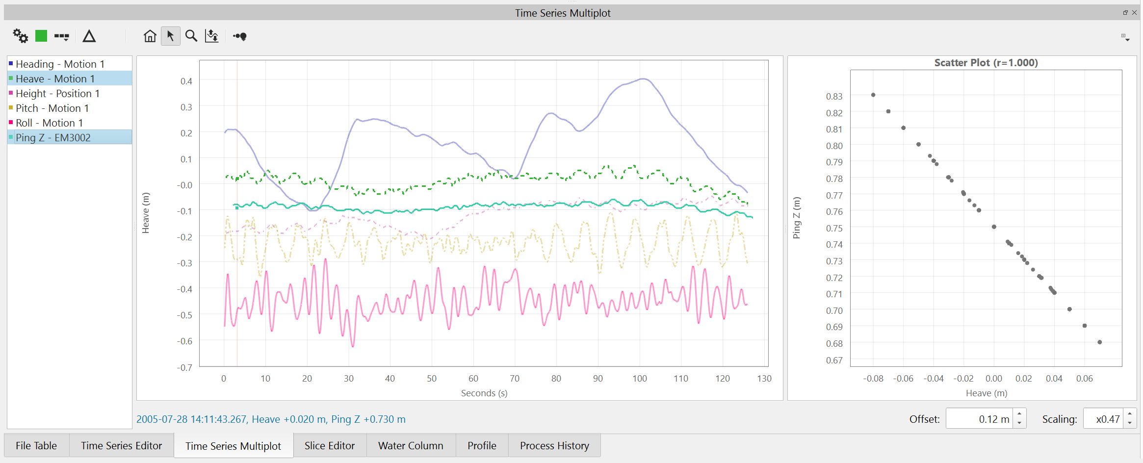
Attributes With High Correlation

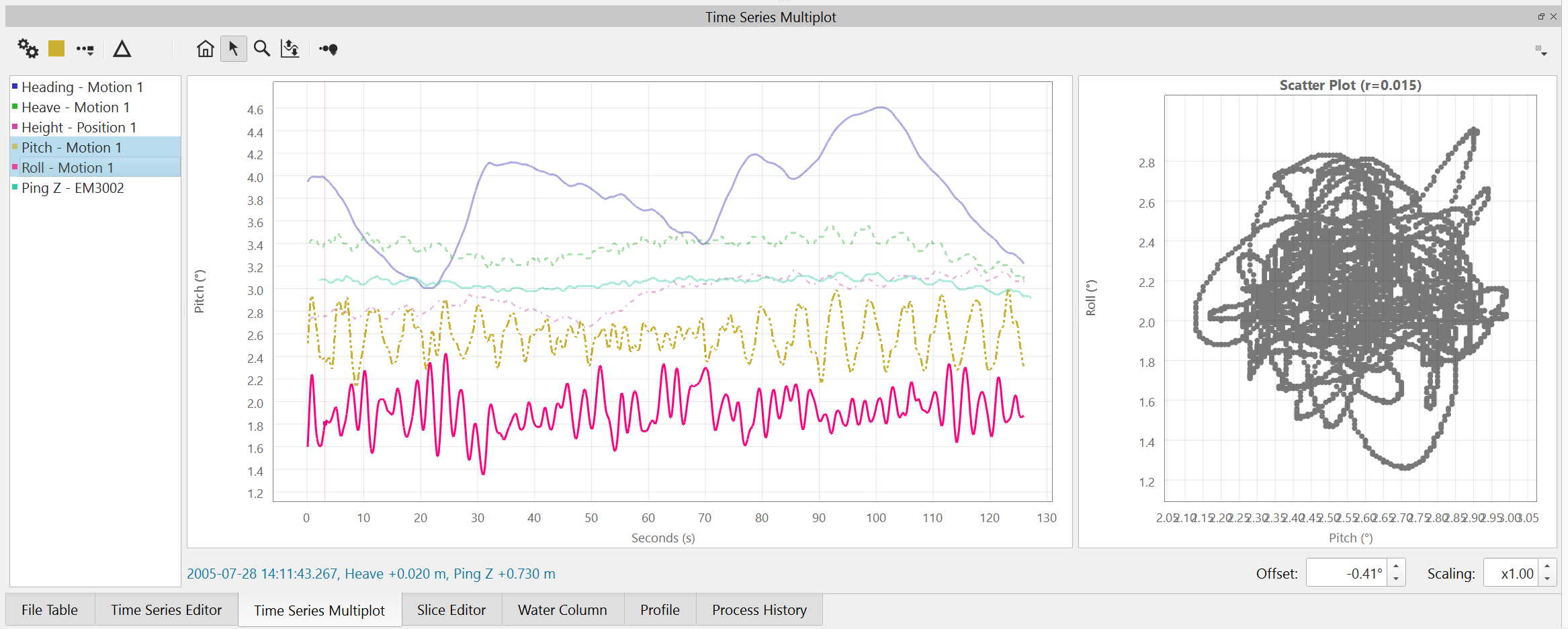
Attributes With Low Correlation

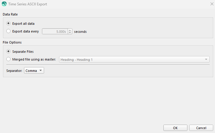
Export to ASCII

This will launch the Time Series ASCII Export dialog shown below. The Data Rate radio buttons allow you to export every time series sample or a sample rate specified by the Export data every spin box. The File Options radio button allows you to create a file per attribute type or to merge all attributes into a multi-column file using the selected attributes as the time master. Attributes other than the time master will be interpolated if they occur at different rates than the master time series. All exported files automatically appear in the ~myproject/Export folder with the naming convention sourcefilename.attribute name. If you decide to merge the data, the filename will be sourcefilename.merged.txt. If you have loaded a Route Layer and additional KP value column will be exported. Commas, spaces or tabs can be selected as separators in the export.

Save Plot To Image

This will save the current Multiplot to an image file. The file type by default is PNG. The default folder is the ~myproject/Export folder. The first image below is the configuration of the Multiplot before export. The next image is the exported image. Notice that Qimera includes the vertical axes of the other attributes as well as a color and line pattern legend.

Multiplot to Export

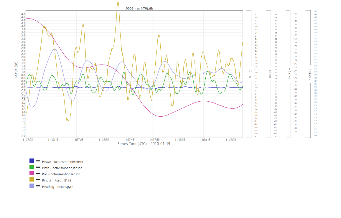
Exported Multiplot Image

Save Scatter Plot to Image

This will save the scatter plot to an image file.

Show Gridlines

This option will show/hide the grid lines in the plot areas.