
How-to TU Delft Sound Speed Inversion
This How-to is a step-by-step description for using TU Delft Sound Speed Inversion tool, available from Qimera 1.6 and up. This tool fixes problems in bathymetric data caused by Sound Speed issues in areas where sound speed in water is challenging, like in estuaries where fresh water meets seawater or near factories where hot and cold water meet.
On this page:
Introduction
QPS has worked together with the Technical University of Delft (TU Delft), The Netherlands to implement their sound speed inversion algorithm in QPS Qimera. The TU Delft algorithm allows for a completely automated refraction error correction.
This algorithm works by taking advantage of the overlap between survey lines, harnessing the power of redundancy of the multiple observations. For a given set of pings, the algorithm simultaneously estimates sound speed corrections for the chosen pings and their neighbors by computing a best-fit solution that minimizes the mismatch in the areas of overlap between lines. To do this the tool uses a simplified model of the water column in which the sound speed throughout the water column is constant from top to bottom (this is essentially the harmonic sound speed) and a refraction correction occurs only at the transducer face to allow for a ray bending correction. The data quality may significantly improve when applying this calculated harmonic Sound speed. For accountability, the algorithm also preserves the output of the inversion process for review, vetting, adjustment and reporting. This process is repeated across the entire spatial area, allowing for an adaptive solution that responds to changes in oceanographic conditions.
The collection of images below depict two examples of where the tool removed the effects of refraction from the data. The set of pictures on the left show where "Smileys" in the data were fixed, and the right pair show an example of "Frowns" being fixed. The top images show a slice of the data before corrections, and the bottom images are from after corrections.
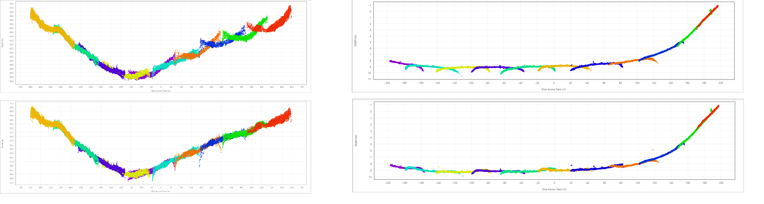
(All images in Slice Editor view, colored by line)
Benefits of this method include:
1. Automated and objective: Overcomes the limitations of other solutions which require manual review and adjustment of the 'fudge factor' corrections that are inherently subjective and NOT repeatable. (even by the same operator!)
2. Physics-Based: Honors the physics of acoustic ray bending.
3. Accountable: Preserves the output of the inversion process for review, vetting, adjustment and reporting. If you don't like the result, you can easily disable it.
Step-by-Step Guide
Step 1 - Assess Your Data
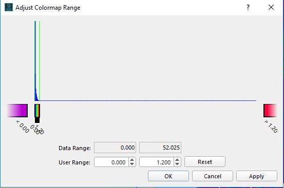
Determine the lines that require Sound Velocity improvement by assessing the data/survey. A good way to visually spot refraction errors in your data is to set the Dynamic Surface attribute 'Color by' to Standard Deviation, and then adjust the colormap to emphasize outliers. The Adjust Colormap Range dialog will come up, you can left-click and right-click on either side of the histogram to adjust the range. You can also type in values in the text entry boxes below.
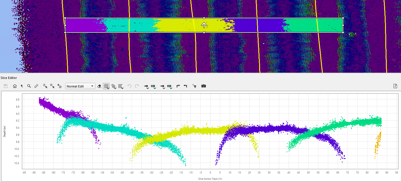
Next, using the Slice Editor (either 2D or 3D), you can zoom to problem areas and color the data by line to check the overlap of adjacent lines. In some cases, all survey lines must be adjusted. In other cases, only a few lines need to be adjusted. If your dataset is not pre-cleaned, cleaning of the data should occur here.
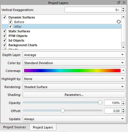
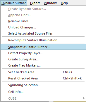
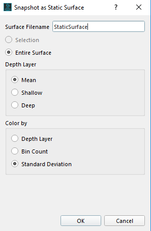
An additional step that can aid in assessing the results of the correction is to create two dynamic surfaces at the beginning of your project, one for before the corrections and one for after. This allows the user to easily see what changed in their data. Alternatively you could snapshot the dynamic surface as a static surface, a function accessed in the Dynamic Surface drop down menu.
Step 2 - Save a Before Image
This second step is not strictly necessary, but is a suggested best practice to help you assess the results of the algorithm by capturing a snapshot of the results before application of the algorithm.
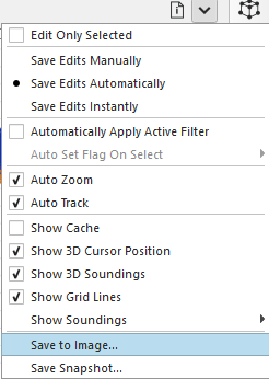
With the 2D slice editor open, and a slice of the data selected, select the "Save to image" option found under the drop down menu in the top right corner of the slice editor window. You will be prompted to give this image a name and location.
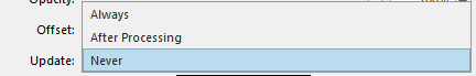
If you followed the optional step to create two dynamic surfaces, once the slice editor image is saved, set the before dynamic surface to never update, so that the refraction corrections are not applied to it. In this way you can compare the two surfaces once the tool has run.
Step 3 - Select The Data That Needs Repair
In the Project Sources Window, select the appropriate line(s) for which you'd like to compute a correction (the left image below). In the Project Layers window, select the Dynamic Surface you'd like to have improved (the right image below).
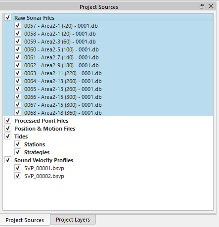
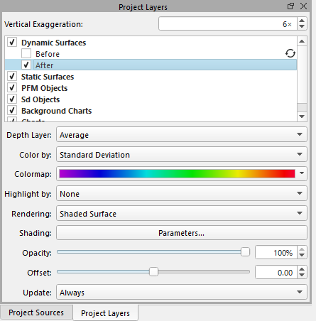
Why do you need to select lines and surfaces? The short answer is that the lines you select will be the lines that are corrected. The Dynamic Surface that you select helps the algorithm determine which neighboring survey lines can be used to assist the algorithm, even if those lines do not need to be corrected. You should only select the lines that you want to repair, the Dynamic Surface's spatial indexing will help the algorithm find the surrounding lines that will assist in the repair. The surrounding lines will NOT be adjusted by the algorithm.
Step 4 - Run The Algorithm
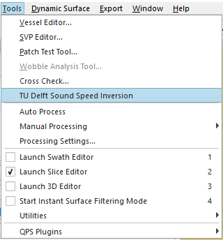
Select the TU Delft Sound Speed inversion tool, available on the Tools drop down menu.
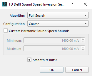
Parameters
There are four parameters which can be set to the users preferences: Algorithm, Configuration, Custom Harmonic Sound Speed Bounds, and Smooth results.
"Algorithm" can be set to either Full Search or Quick Search. There are pros and cons to each method:
| Algorithm | Optimization Method | Speed | Best used for | Other |
|---|---|---|---|---|
| Quick Search | Nonlinear Least Squares | Fast to Medium |
| Easily distracted by noise and terrain |
| Full Search | Differential Evolution | Medium to slow |
| Reliably finds best solution |
"Configuration" can be set to Coarse, Fine, or Very Fine.
Generally the Coarse setting is sufficient in most cases, however there are a couple other factors to consider:
| Configuration | % of Data used | Speed | Best used for |
|---|---|---|---|
| Coarse | 25% | Fastest | Environments with gradual change in sound speed. |
| Fine | 50% | Medium | Environments with less gradual, but not abrupt changes in sound speed. |
| Very Fine | 100% | Slowest | Environments where very abrupt changes in sound speed are expected. |
Enabling this option will make a weighted moving average of the resulting harmonic sound speed time series. This is most beneficial for the Quick Search which is more prone to poor estimates in noisy environments.
"Custom Harmonic Sound Speed Bounds" gives the option to limit the sound speeds used by the tool.
"Smooth results" can be toggled on and off. Enabling this option will make a weighted moving average of the resulting harmonic sound speed time series. This is most beneficial for the Quick Search which is more prone to poor estimates in noisy environments.
Step 5 - Assess Your Results
This step is not strictly necessary either, but it is a good practice to verify your results.
The reprocessing of the sounding results that occurs after completion of the algorithm run in Step 4 will trigger the automatic update of any Dynamic Surfaces that use the selected lines (unless set to never update). This is why it is helpful to have a Snapshot surface first, you can compare the results before and after the tool is run. You can check for the improvements of the Dynamic Surface by comparing to the 'Before' Dynamic Surface or Static surface snapshot taken from the Dynamic Surface at step 2. The most common way to do this is to compute a surface difference.
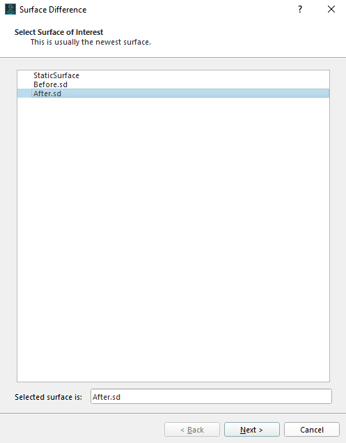
Select your 'Before' Dynamic Surface or Static Surface computed in Step 2, and also select your newly updated Dynamic Surface.
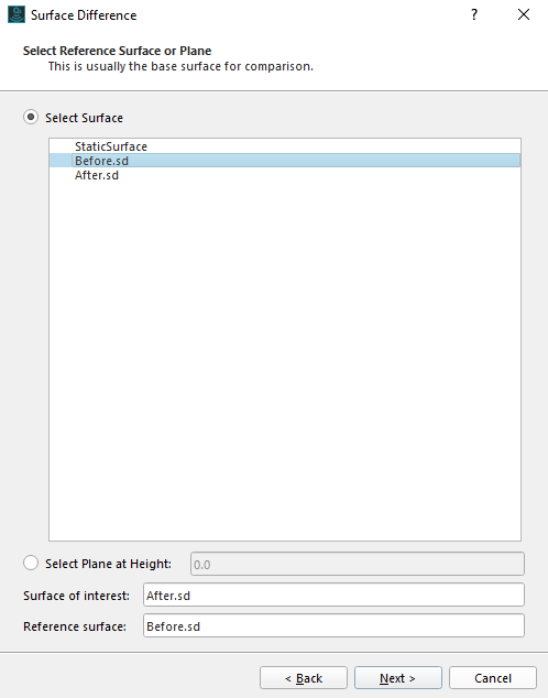
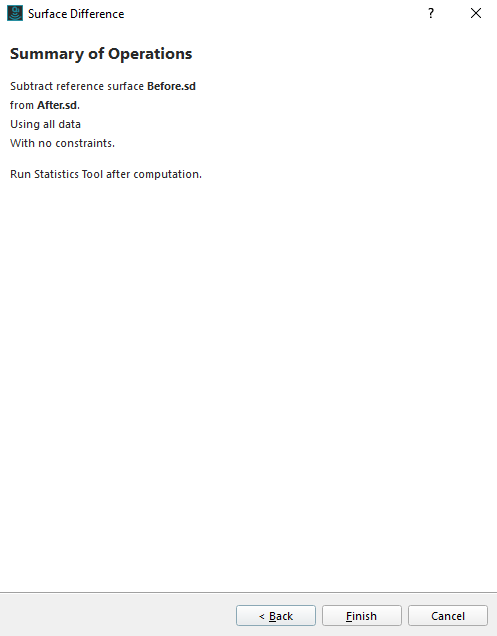
Under the Layers menu, choose the "Surface Difference..." option. This will launch a wizard that will walk you through the process of creating a surface difference. The first stage of the wizard is shown below, typically at this step you choose the Dynamic Surface since it is the "new" surface that you want to compare against the original surface. In the second step, you would typically choose the Static Surface that you created in Step 2.
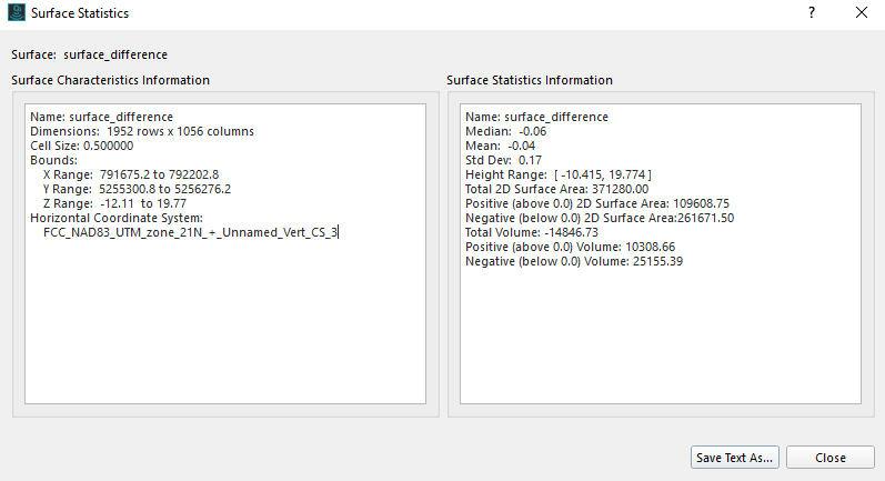
At the end of the process, it will give some statistical results which can be saved as a report, see below for an example.
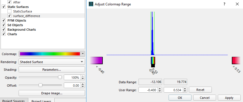
You can review the surface difference map and assess the outcome by adjusting the histogram and colormap to help emphasize areas where there are large differences between the original data and the corrected data. Start by selecting the surface difference result from the Project Layers window, and then click on the Colormap below it and select "Adjust Colormap Range". The Adjust Colormap Range dialog will come up, you can left-click and right-click on either side of the histogram to adjust the range. You can also type in values in the text entry boxes below.
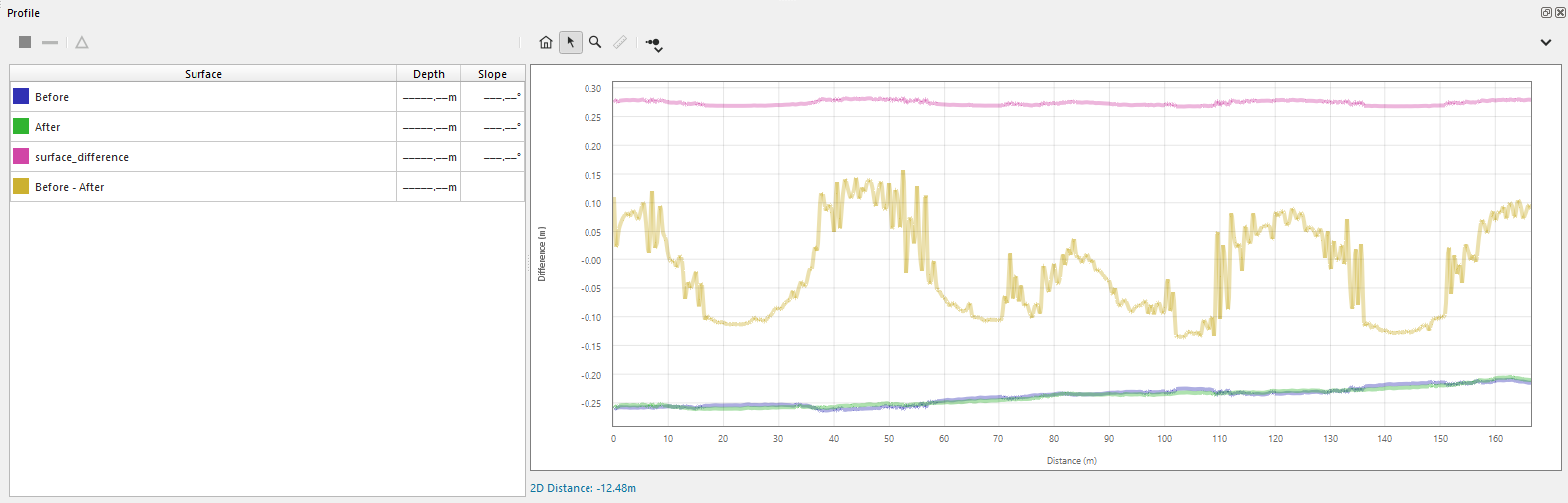
Now that you have improved the contrast of the surface difference result, you can profile in the surface for areas where large differences are seen to assess the magnitude of the difference. A profile can be done with a right-click and drag, or by switching to profiling mode. Additionally, a difference series can be computed in the profile view by selecting the two surfaces you wish to see the difference between, and then the tool is accessed by the triangle button in the top left of the profile window.
Step 6 - Make Adjustments if Necessary
You can review the algorithm's output of Harmonic Sound Speed in the in the Time Series Editor.
In case you're not sure about the improvement or if you wish to try the other algorithm settings for the sake of comparison, you can re-run the TU Delft Sound Speed Inversion tool GUI and choose different settings like Quick Search, etc. This calculates a new harmonic sound speed time-series result, which can be reviewed and compared to the harmonic sound speed previously calculated. You can view the different results this in Time Series Editor.
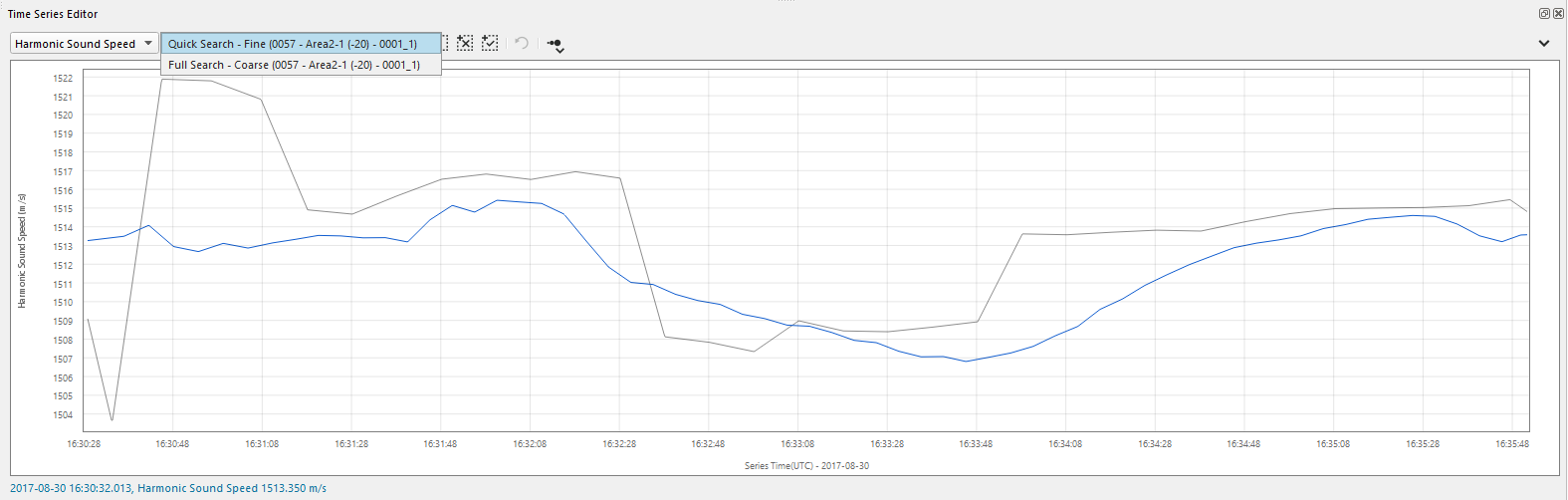
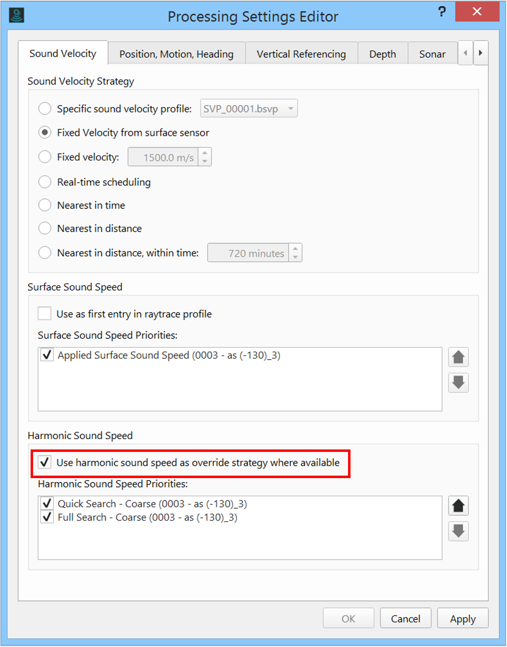
The results from the last run of the tool will be the one that is used in any follow up processing. If you want to adjust which result you want to use after your investigation, you can manage which results you prefer to use in the Processing Settings dialog under the Tools drop down. Select the time-series you prefer and move it to the top of the priority list and click Ok. The data will be reprocessed and the Dynamic Surface will update.
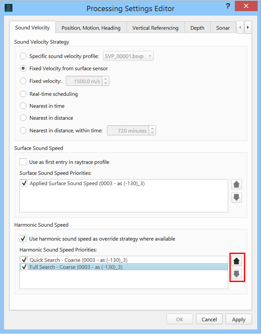
If you are not happy with the results or you need to disable their use, you can do this by unchecking the tick box over the Harmonic Sound Speed time-series items, as shown below.
For a more in depth explanation of specific options within this tool, visit our reference page: TU Delft Sound Speed Inversion Settings Dialog
References
For the interested user, there are two publications that describe the underlying algorithm.