
Getting Started
This article will help you set up a Qimera project.
For Installation information, please see How-to Install Qimera and How-to License Installation (Qimera 1.5.7 or older) or How-to Qimera - License Manager (1.6.0 and later)
Getting up and running with Qimera begins with creating a Project, or opening an existing Qinsy project. Qimera projects store bathymetry data in QPD format and external source data such as SVP, vessel and tide; they also allow you to manage your data processing flow and preserve any processing steps that you have already accomplished, and provide a centralized location for storing exported products. The data used for this Quickstart is Kongsberg EM2040 single head data from Wellington, New Zealand and was part of the Shallow Survey 2012 common dataset; these files are available for download. These files are Raw Sonar Files and when using Qimera they can be fully processed.
This Quickstart demonstrates a straightforward workflow with one of the more comprehensive data types, Kongsberg .ALL files. Other data types will follow a similar workflow, but there may be additional steps or you may encounter other dialog boxes that are not shown in this Quickstart. For other data types, we have created How-to's that attempt to document differences in workflow. The available How-tos are: How-to Work with Qinsy Data, How-to Work with Hypack HSX Data, and How-to Work with Kongsberg ALL Data (links back to this page, and provides info, hints, and tips specific to Kongsberg ALL data).
The import and processing of raw data formats is dependent on licensing. In Qimera, go to the Help drop-down menu and choose View License Status to view your current license coverage.
On this page:
We have implemented a new option to change default left mouse button behavior based on workshop feedback with former Qloud users. The default left mouse button will remain the same in that you need to hold down the Shift key to adjust the view in the Scene when you are in another mode such as polygon selection. The new optional mode leaves the left mouse button always in navigation mode and you hold down shift to activate the secondary mode, such as to draw a polygon. Many Qloud users have found this second mode more intuitive in that you can draw a selection and then it remains where you drew it when you attempt to adjust the 3D view. This setting is available in the 'General' tab of the Qimera Preferences.
Quickstart Info
You can view a full-size version of any image in this Quickstart by clicking on the image. Numbers in images are referred to in the text preceding the image or in the image caption itself. Blue text indicates a link to the manual, another document, or data.
Step 1 – Launch Qimera
Launch Qimera by clicking on the icon, or from the applications menu of your computer (using Windows: Start > All Programs > QPS > Qimera).
![]()
Step 2 – Create the Project
Qimera provides a guided Dynamic Workflow that can guide you through processing steps and will attempt to complete certain steps (such as vessel extraction, for example) for you. Part of the Dynamic Workflow is the Welcome Screen, which will launch automatically when Qimera is opened. From the Welcome Screen, select New Project.
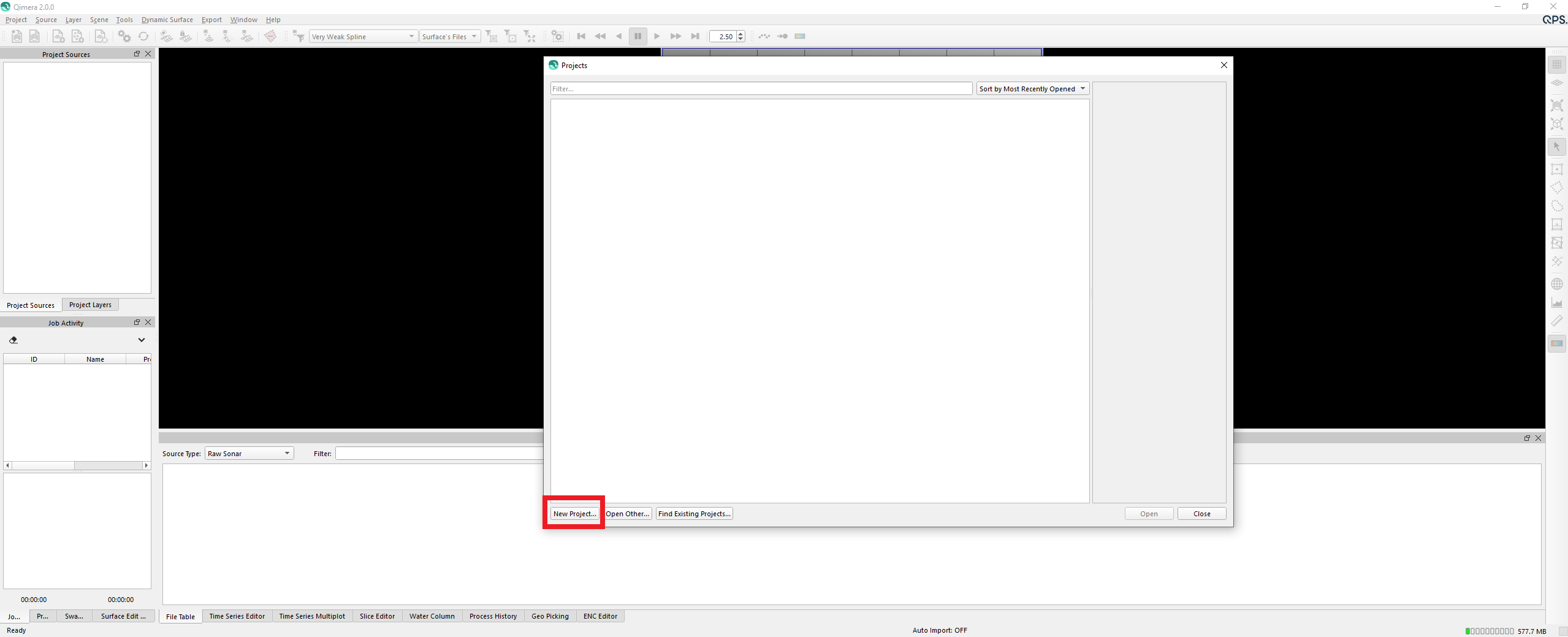
Qimera Welcome Screen
The Create Project dialog will launch. Add project name information (1). By default, the folder for your project will be in the '/Users/username/FMData/Projects' directory (2), though you can choose any location. Once created, the project folder will contain sub-folders for storing bathymetry files in QPD format, internal metadata, extracted external source data, and products. The Description box (3) can be used to add additional notes about the project. Finally, the default ("Automatic" option) is for Qimera to automatically set the project coordinate system based on the first imported line of source data (4). For unprojected/geographic source data, the closest UTM zone will be used; for projected data, the project projection will match that of the source data as set by the user on import. If you prefer, you can select the Manual radial button and manually select a different projection.
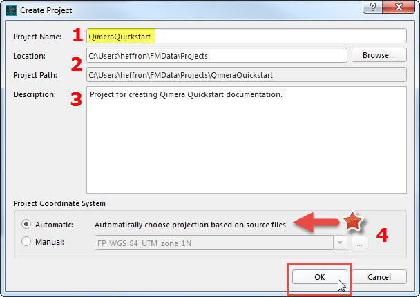
Create Project Dialog
Create Project
Alternatively, you can create a project by clicking the Create Project Button 
Project Projection
At this time, Qimera projects must be projected.
Step 3 – Add Source Files
Qimera provides tools for full bathymetric processing of Raw Sonar Files such as Qinsy DB, Kongsberg ALL, Reson S7K, Hypack HSX, GSF Files, and Edge Tech Files JSF. Qimera can also do limited geospatial processing of Processed Point Files such as ASCII XYZ, Hypack HS2, and Danish Hydrographic FAU. A list of Supported Data Formats can be found here.
The guided workflow will next ask you if you would like to add source files to your new project. Choose Add Raw Sonar Files.
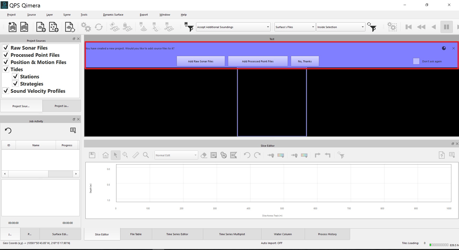
Add Source Files prompt.
Add Source Files
Alternatively, you can add Raw Sonar Source Files by clicking the Add Raw Sonar File button 
The user will then be presented with Add Raw Sonar Files dialog shown below. This dialog lets you select specific files or a directory containing your files. Here, we choose Add Files (1) and add the raw sonar files. Set the coordinate system of the imported data (2). Click OK to start the add files process (3).
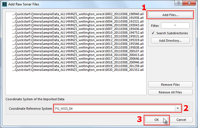
Add Files Wizard
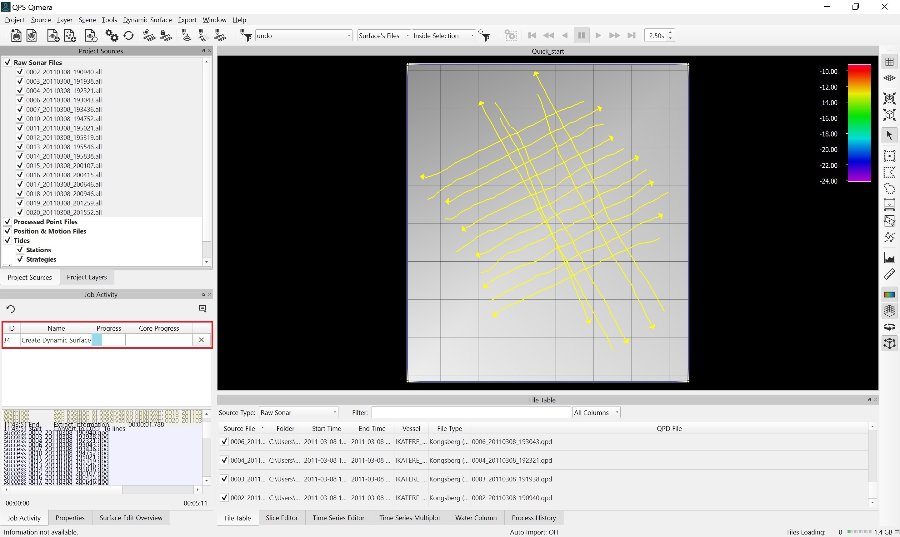
Qimera attempts to automatically detect and extract any available information as it adds source files to the project. Extracted information includes vessel configuration, position, heading, motion, sound velocity, and tide and/or GPS/GNSS height corrections – if it is supported by the file format and available in the file (for a full list of what is extracted from each supported format, click here). Multibeam records are indexed and retrieved as necessary from the raw files; only minimal metadata information is extracted from the multibeam ping records. Rich formats will contain much of this information, making your processing workflow faster. Other formats may be missing this information, in which case it will have to be added separately.
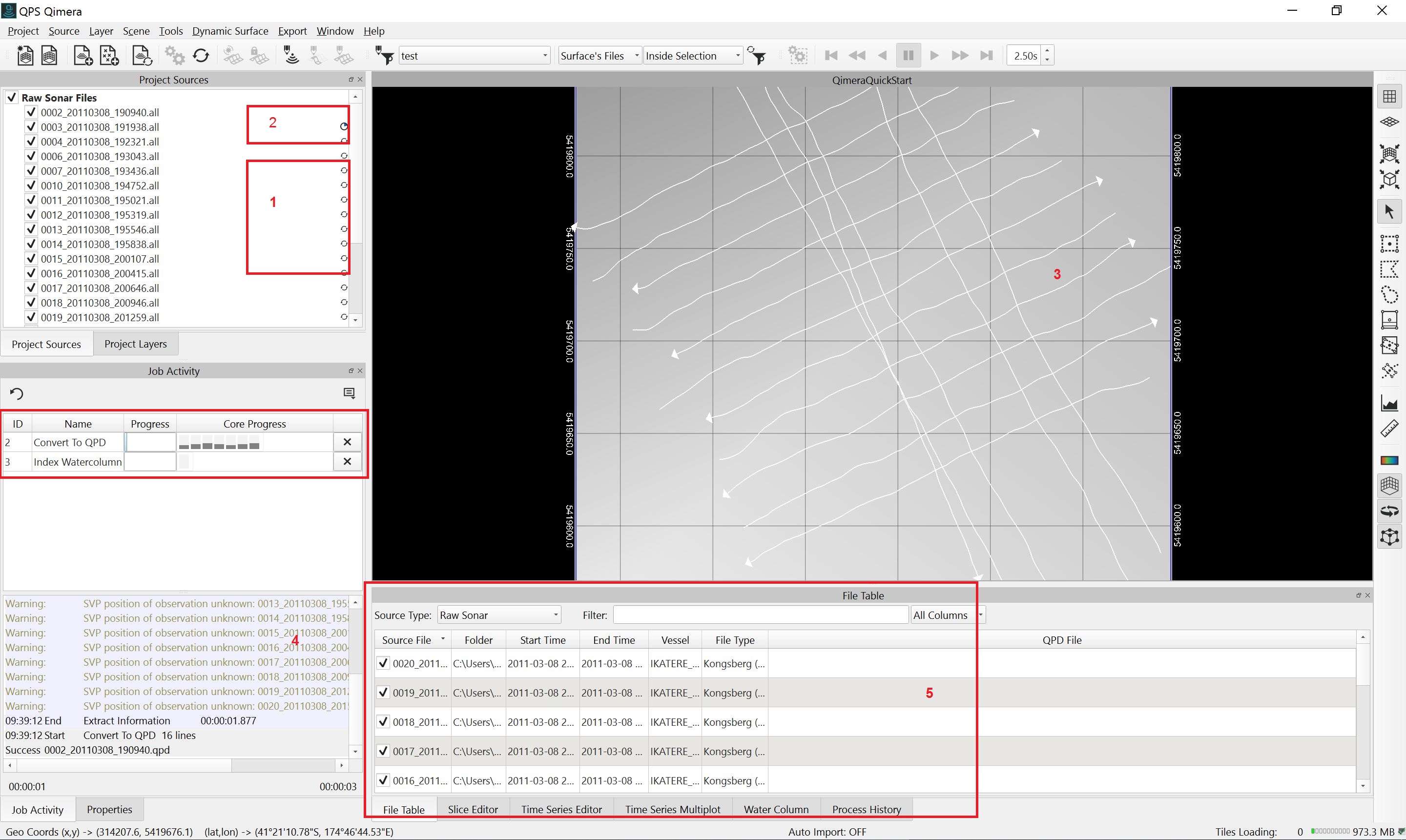
Information being extracted from files during import. Individual file load progress is shown (1) and after each file loads the processing status is indicated (2) and a trackline is drawn (3). Overall progress is monitored (4), and information that is extracted populates the File Table view (5).
As the extraction progresses, Qimera will track processing and any potential issues or errors in the Job Activity Window.
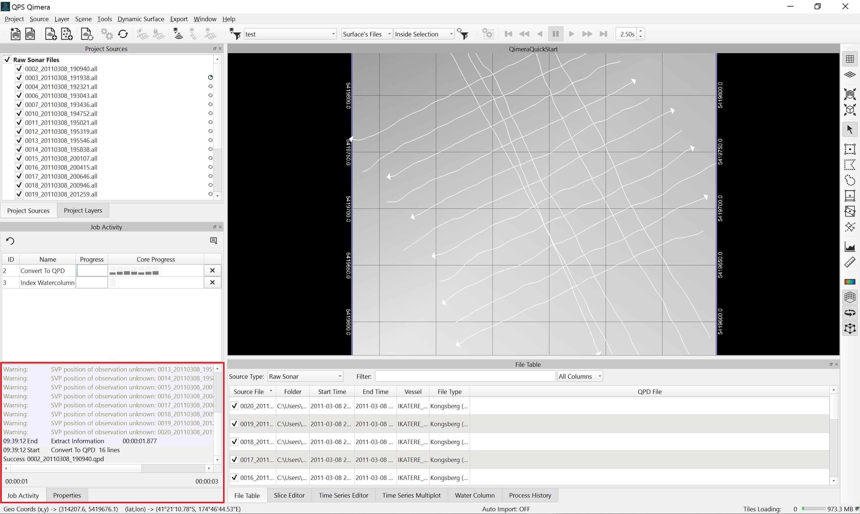
Job Activity Window showing processing stage, warnings, and errors encountered during load.
As information is extracted from the source files, it is written to the Qimera project.
For rich formats with soundings (XYZ footprints calculated during acquisition or online), Qimera can directly convert the online XYZ for each file during import and write them to a QPD, which is the the QPS internal format for processed point data. The QPD files are then written to the project. Currently, this process is only possible with Kongsberg .ALL data and .GSF files.
For acquisition by Qinsy users, the QPDs computed while online are used directly without recomputing. For file formats that contain complete sonar information and all supporting ancillary data, Qimera can calculate XYZ footprints for each file after import and write it to a QPD.
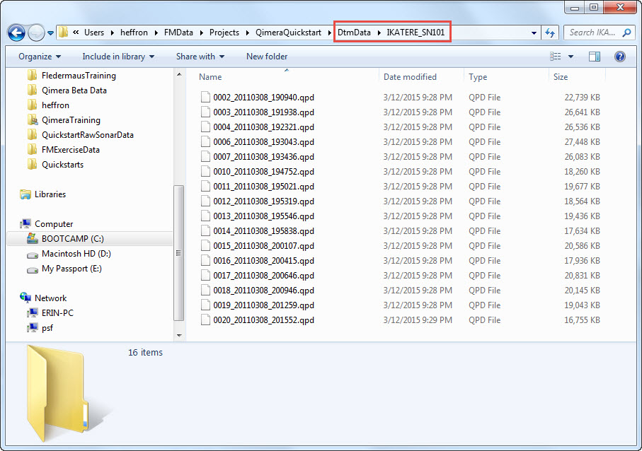
QPD files generated for the source files.
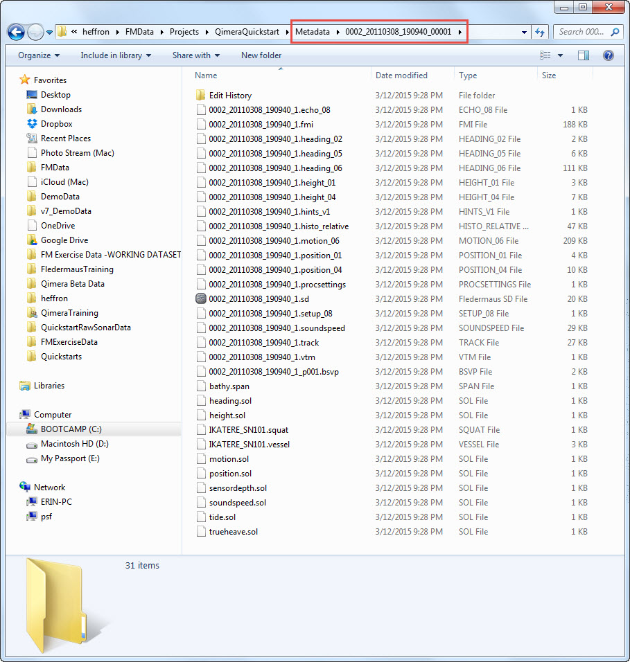
Extracted information for one source file line in the Metadata folder.
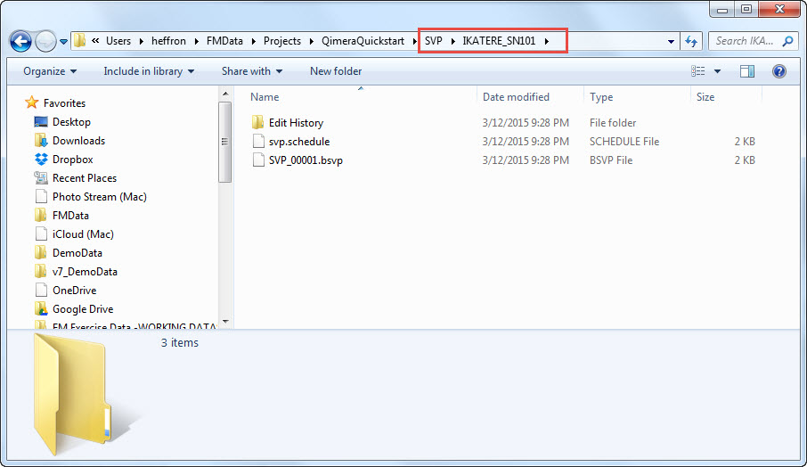
Extracted SVP information in the SVP folder.
If water column data is available in the files, it will be indexed as well.
The source files for the project will be listed in the Project Sources Window, under the Raw Sonar Files (which is the Parent level) navigation track lines will also be visible. The check boxes next to each line control visibility in 4D Scene; lines that are checked are visible. Source file location and the QPD file that corresponds to each source file can be viewed in the File Table Window.
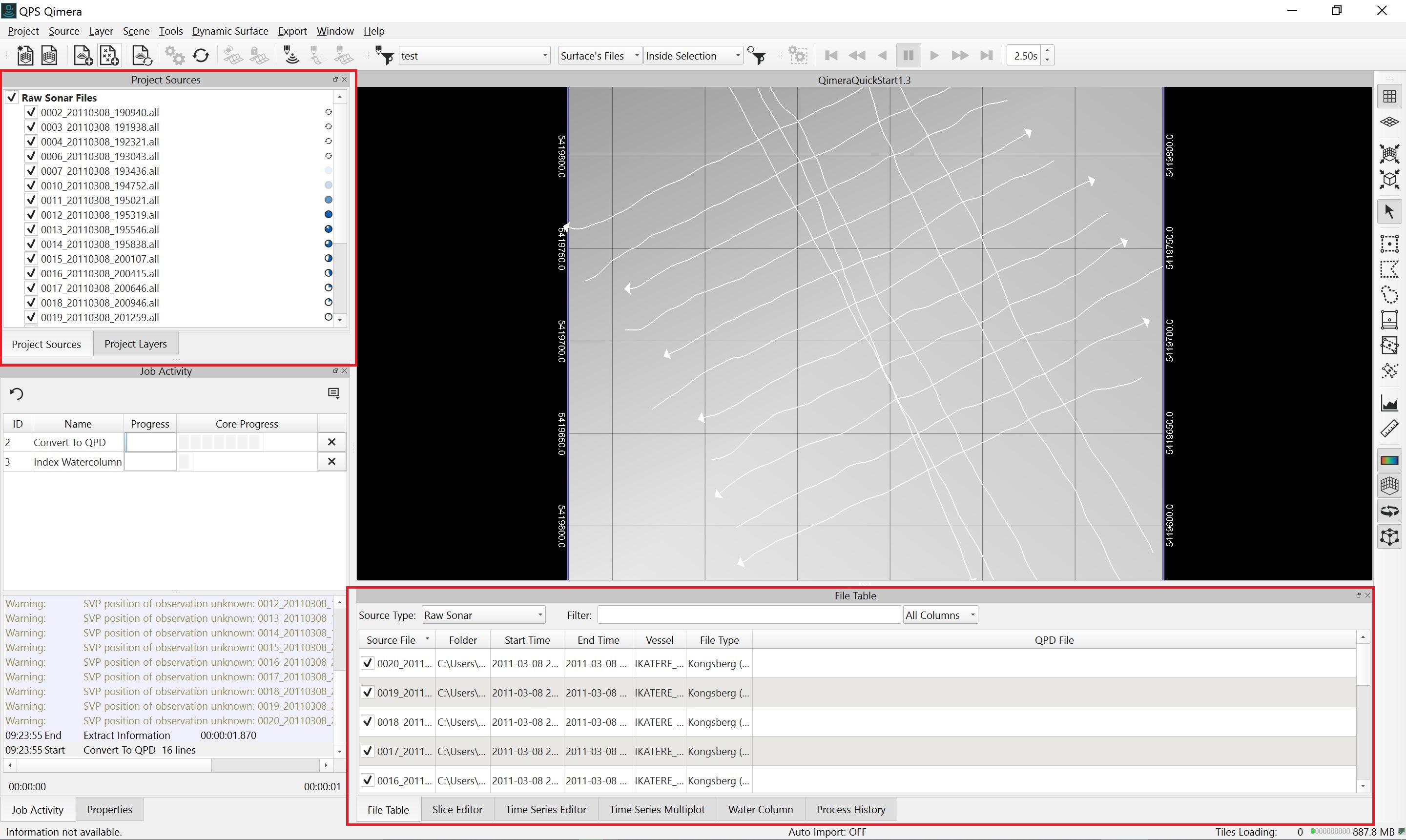
Files Loaded and visible in Project Sources , File Table , and 4D Scene.
File Visualization & Selection in Qimera
Checking a file on 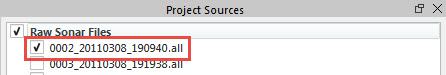
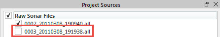
For files to be used in a processing routine (such as surface creation), they can be checked on or off, but they must be selected in order to be processed 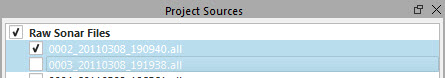
This is a key part of Qimera's workflow. For an overview of the Qimera user interface, click here.
Note: When lines have just been added to your project and you are prompted to do a process, all of the lines that were added will automatically be included in that process.
Step 4 – Create Dynamic Surface
Additional Processing
Some file formats may need additional source information and/or source files and should have additional processing applied before creation of the Dynamic Surface. This will be indicated by a prompt (for example, a message that your vessel offsets are zero and prompting you to add information) and/or by the 
Once the files have loaded, Qimera will prompt you that lines have become ready for cleaning, and ask whether you would like to add them to a Dynamic Surface. Dynamic Surfaces are gridded bathymetric surface models that can be viewed and edited in 2D or 3D; they are "dynamic" because they reflect the state of the processed data (the QPD files) and will update to reflect changes you make during various processing steps. Click Create New in the Dynamic Workflow prompt in 4D Scene to start building your Dynamic Surface. Alternately, if the Dynamic Workflow does not activate, a new Dynamic Surface can be created by selecting from the main toolbar Dynamic Surface → Create Dynamic Surface.
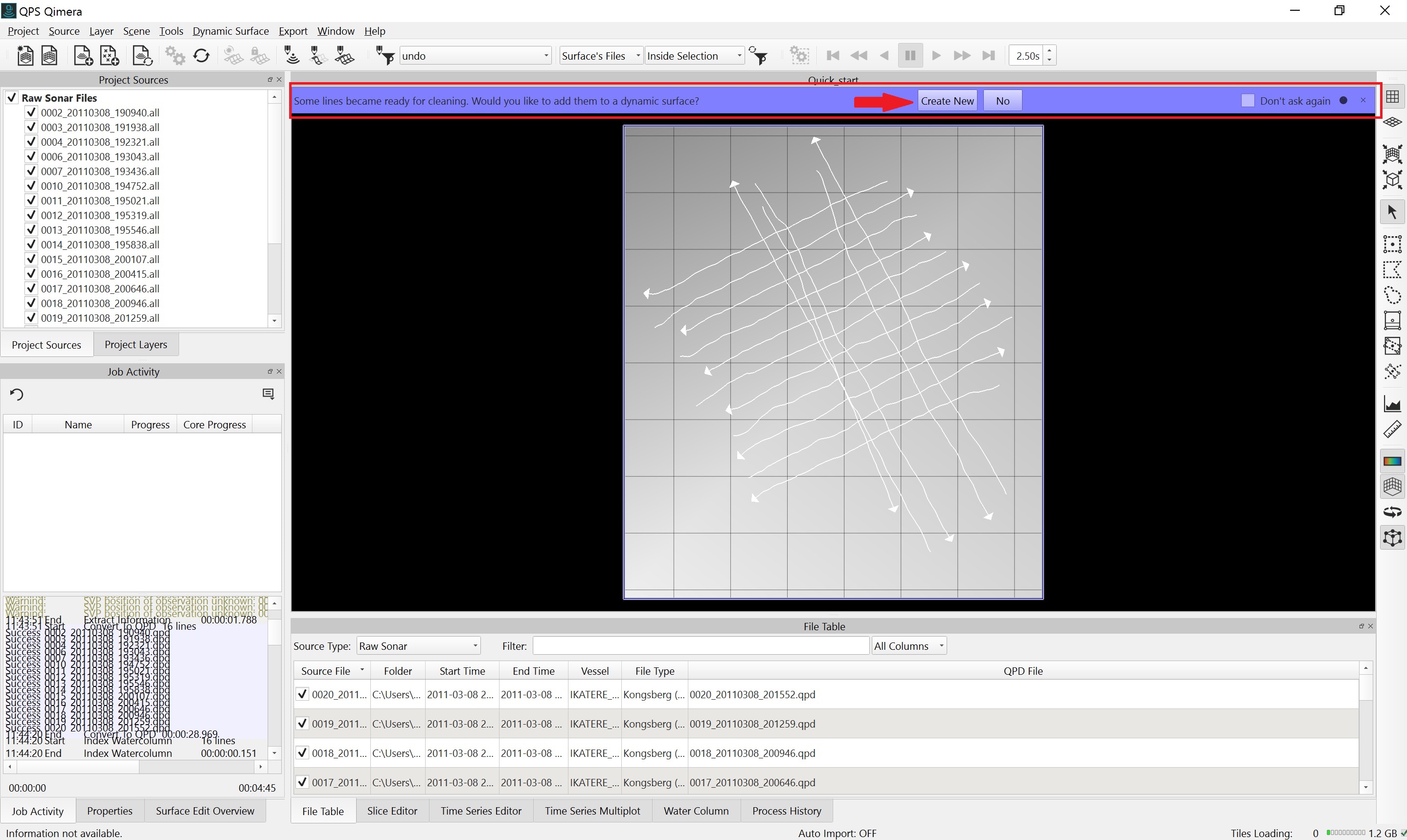
Add lines and Create New Dynamic Surface prompt. (Dynamic Workflow)
The Create Dynamic Surface Dialog will launch. Change the name of the surface if desired (1). Qimera will calculate a suggested cell size using an approach based on the footprint size of an average multibeam echosounder projected to the mean depth of the set of files provided to the wizard (2), though you can adjust the value. If you would like to create a CUBE surface, check on Enable CUBE Grid (3) and adjust the CUBE options by clicking on Settings (4). Click OK to start the surface build. Link to what CUBE surface is?
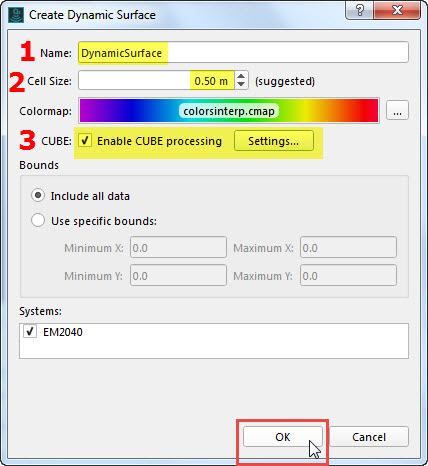
Create Dynamic Surface dialog.
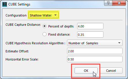
CUBE Setting Dialog. Choosing a Configuration will auto-fill the CUBE Capture Distance, Estimate Offset, and Horizontal Error Scale; choose Custom to input your own settings.
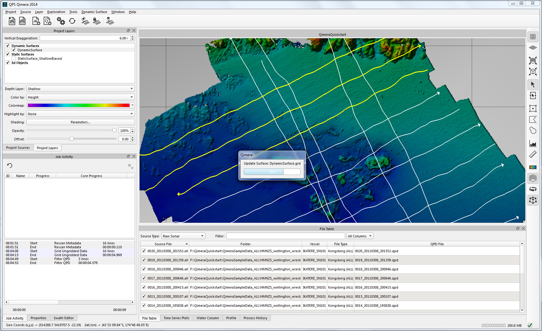
Progress of the build can be followed in the Job Activity Window.
Dynamic Surface build progress.
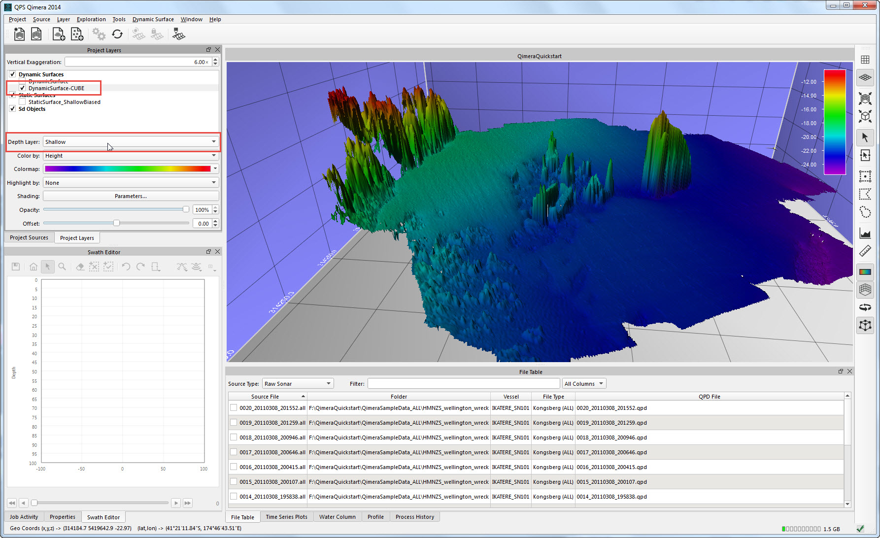
Once the surface build is complete, the Dynamic Surface will be visible in the 4D Scene. If you click on the Project Layers tab, the layer will be listed in the Project Layers Window under Dynamic Surfaces. Selecting that layer (by clicking on it with your mouse) will show attributes for that surface, including the depth layer being displayed, the Color By options for the surface, the selected Colormap, and Opacity controls. At this point, you might choose to turn off your navigation tracklines to get a better look at the surface. You can do this by returning to the Project Sources tab and unchecking Raw Sonar Files.
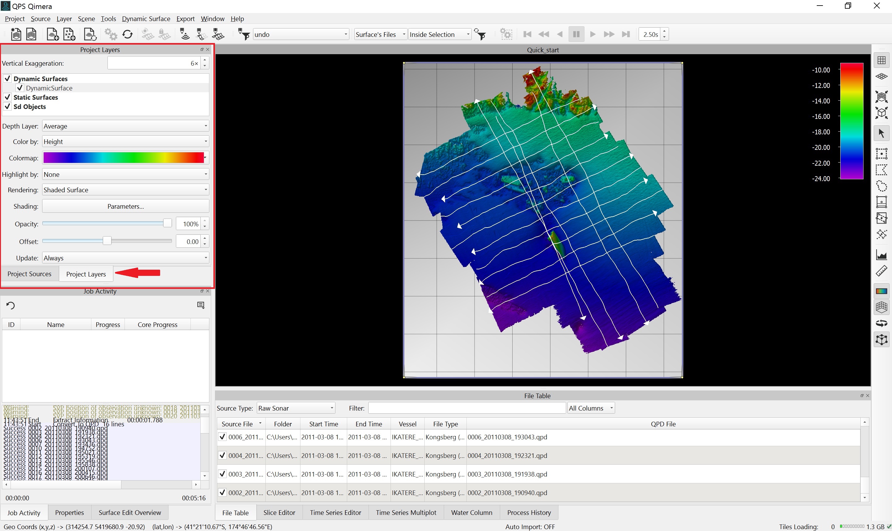
Dynamic Surface.
Create Dynamic Surface
Alternatively, you can create a Dynamic Surface by selecting the files or area of interest and clicking the Create Dynamic Surface Button 
Step 5 – Explore your data
When you start working in Qimera, you will be looking down at your data in Plan View (this button is currently called 2D view) 

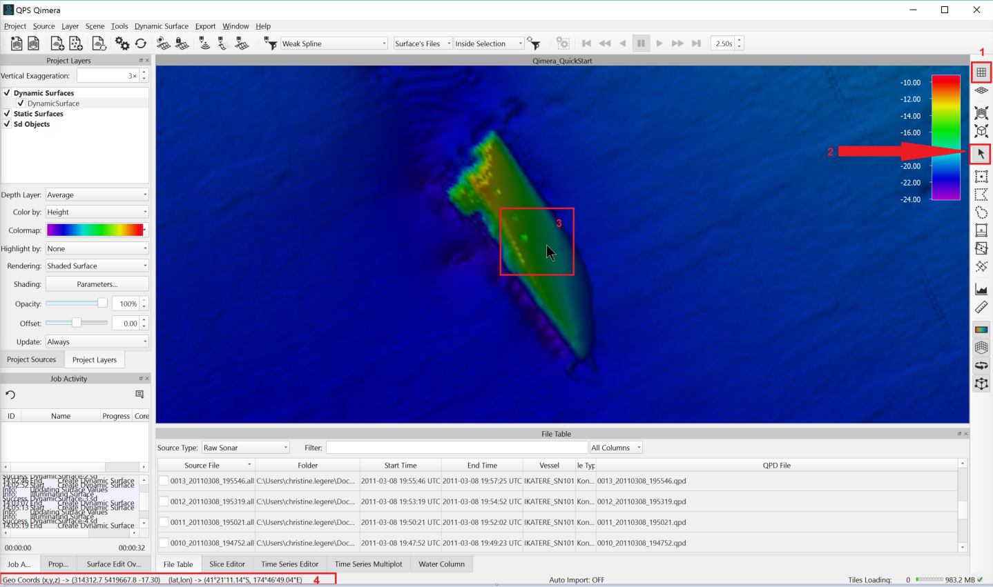
Navigating in Plan View.
Changing to Turntable View 
When working in Turntable View, you may want to adjust your vertical exaggeration (5). This can be done in the Project Layers Window; simply type a new value into the Vertical Exaggeration field. You may also want to turn off the Widgets; this can be accomplished by clicking the View Widgets 
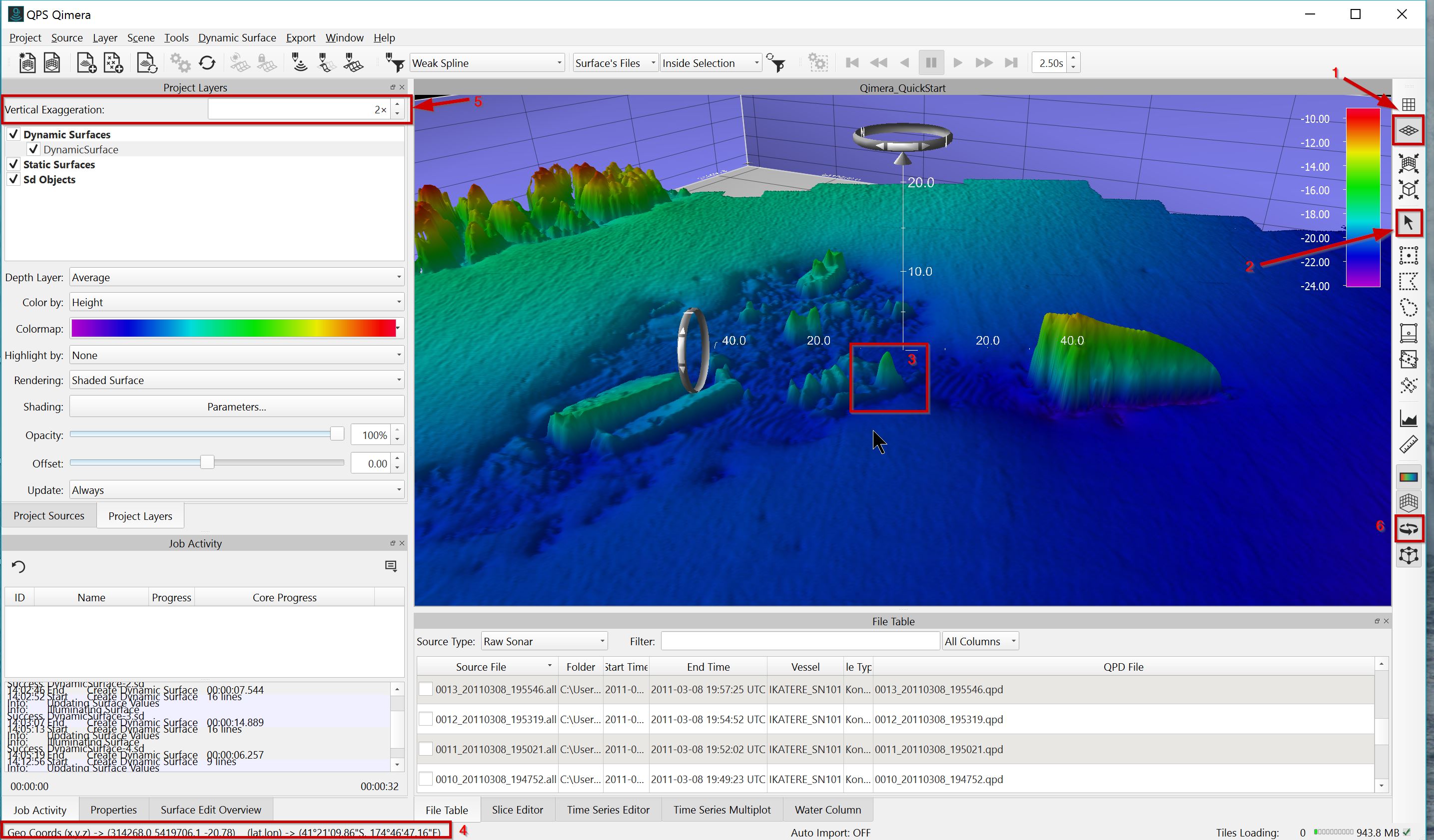
Navigating in Turntable View.
Navigating in Qimera
It is strongly advised that you use a 3 button mouse to work in Qimera. It greatly improves your ability to move quickly through the data.
Step 6 – Add Vessel Information & Adjust for Motion
Patch Test
If you have not yet conducted a patch test in order to determine your motion offsets, do so now and if possible add the information in to your online systems so that motion artifacts are corrected online for any additional data you will be collecting. Offset values calculated using the Patch Test tool can be added to the project from the Patch Test dialog using Add Calibration, Save, and Apply. You can find more information on the Qimera Patch Test tool here, and a howto on using the tool can be found here.
Static Surfaces
You may find it useful to create a Static Surface prior to performing processing steps, to use as a way of comparing the pre- and post- processing results. You can create a Static Surface using the Create Static Surface 
In some cases, the vessel offsets and motion information may not have been populated online. This information can be added in the Vessel Editor. If no vessel offsets or motion information is detected when the sources files are added, you will get a warning that the vessel offsets are zero, and Qimera will ask you if you want to edit the vessel information.
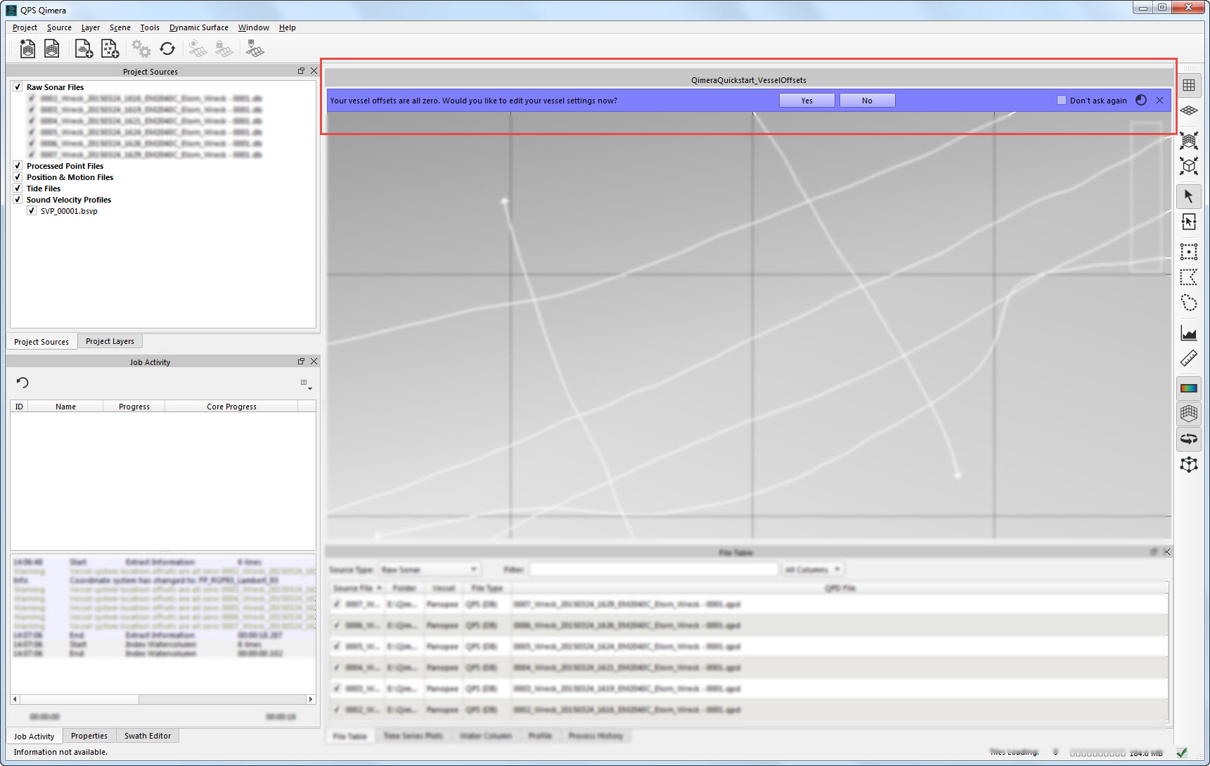
Vessel Offsets warning.
Click Yes to launch the Vessel Editor. Select the system you want to edit form the Systems tab (1). Double click on any of the boxes (2) to make the values editable, then add your offset values.
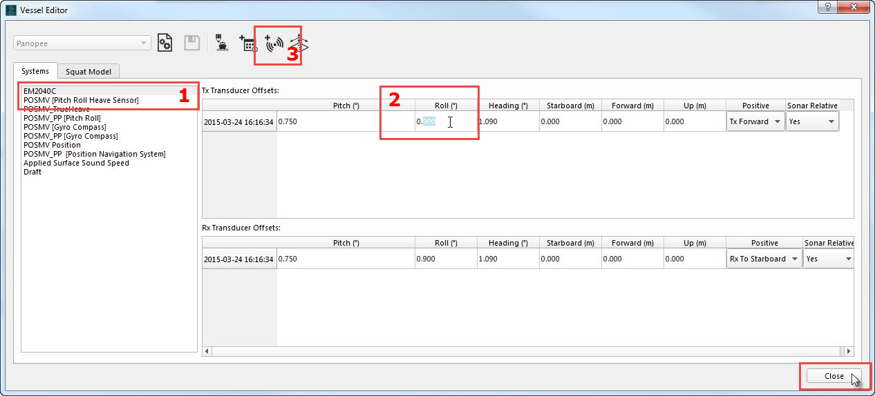
Entering offsets in the Vessel Editor.
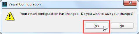
Saving changes to Vessel Configuration.
Re-process your files and recreate the Dynamic Surface to incorporate the changes.
Zero Vessel Offsets
Vessel Offsets may be zero because corrections were applied in the POS MV, in which case vessel offset information won't need to be added. This will depend on your acquisition set-up.
Vessel Editor
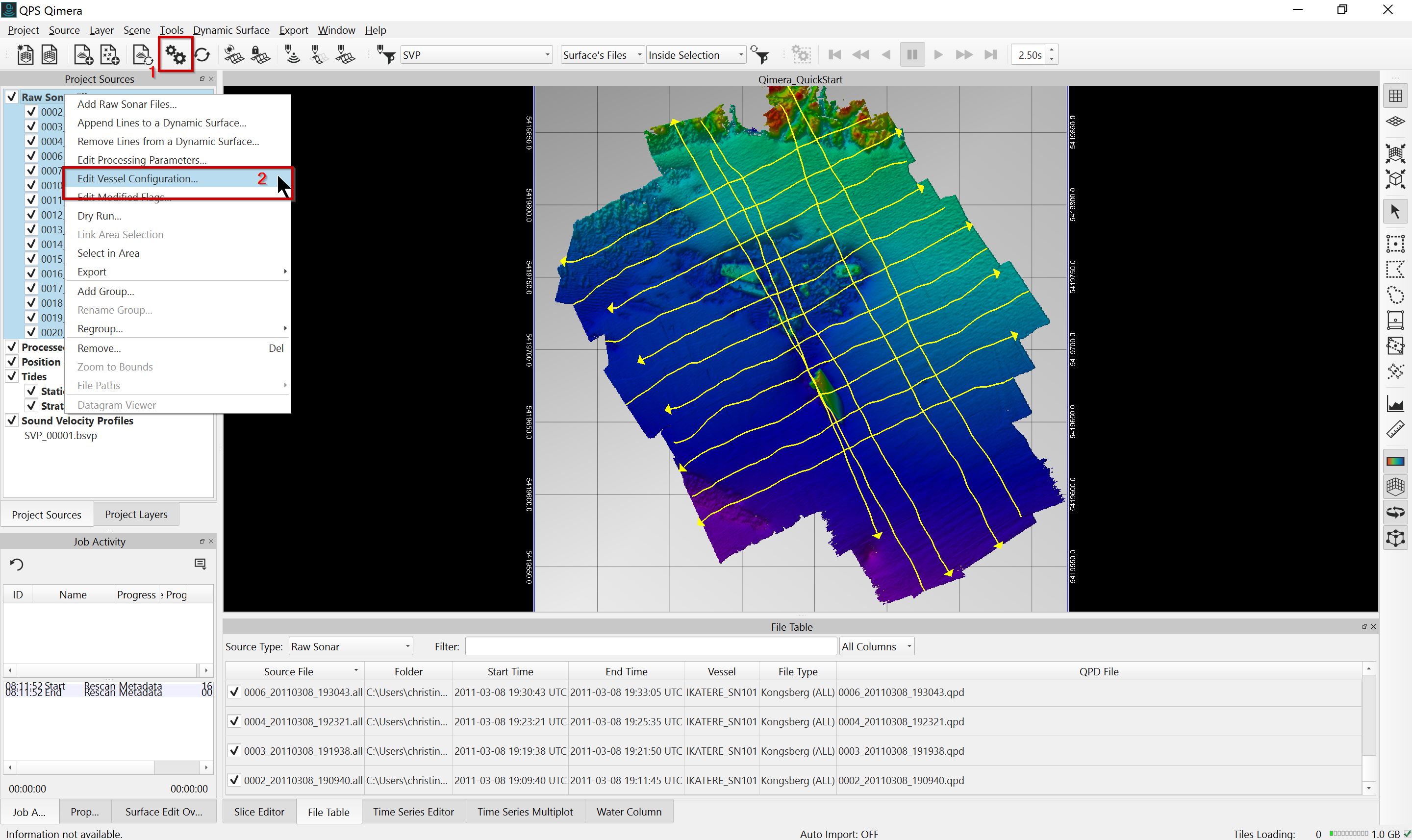
You can also launch the Vessel Editor by right-clicking on Raw Sonar Files in your Project Sources and selecting Edit Vessel Configuration, or by going to the Tools menu and selecting Edit Vessel.
Step 7 – Add Additional Source Files & Perform Processing
Static Surfaces
You may find it useful to create a Static Surface prior to performing processing steps, to use as a way of comparing the pre- and post- processing results. You can create a Static Surface using the Create Static Surface
In some cases, the Raw Sonar File formats do not have all of the information stored in them for full processing – for example, Sound Velocity information is stored in Kongsberg ALL files but may or may not be present in DB, HSX, or S7K files. In other cases you may want to reprocess the position and motion using a different data source.
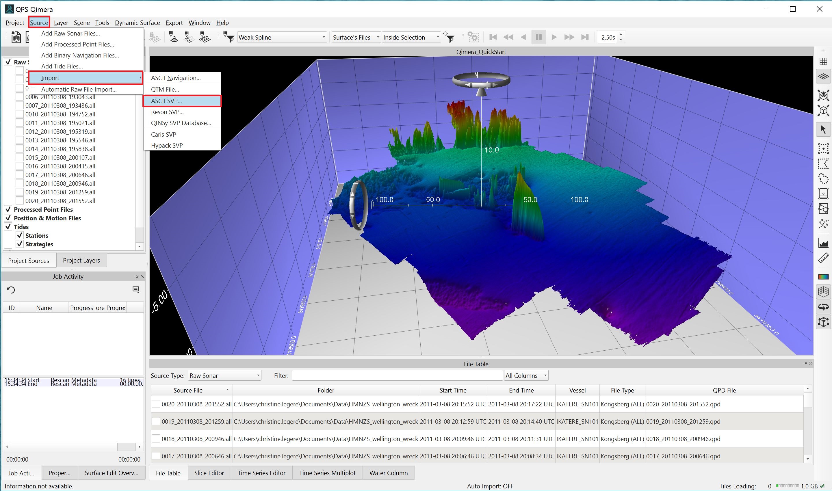
Add & Edit Sound Velocity Profiles (SVPs)
ASCII, Hypack, and Caris SVP information can be added to Qimera by going to the Source menu and selecting Import > ASCII SVP, Import > Caris SVP, or Import > Hypack SVP.
Adding SVP information to Qimera.
Once the SVP information has been added to the project (either via automatic extraction or through the Source > Import menu option) it will be listed in the Project Sources Window under Sound Velocity Profiles.
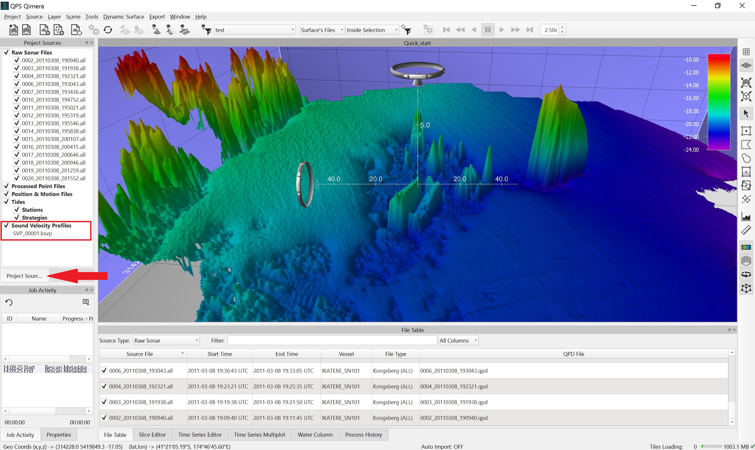
Sound Velocity Profile in Project Sources.
SVP information that is part of the source data will be used for processing and creation of the Dynamic Surface from the beginning. Otherwise, the addition of new or additional SVP information will require manual intervention to link the newly imported SVP files to be applied to particular raw source files. This is done by editing the Sound Velocity Strategy in the Processing Settings Editor for all raw multibeam source items that require updating (accessing the Processing Settings Editor is described below).
Once SVP information is added to the project, it can be edited using the SVP Editor. Launch the SVP Editor by going to the Tools menu item and selecting Edit SVP, or by selecting the SVP of interest from the Project Sources Window, right-clicking, and choosing Edit SVP.
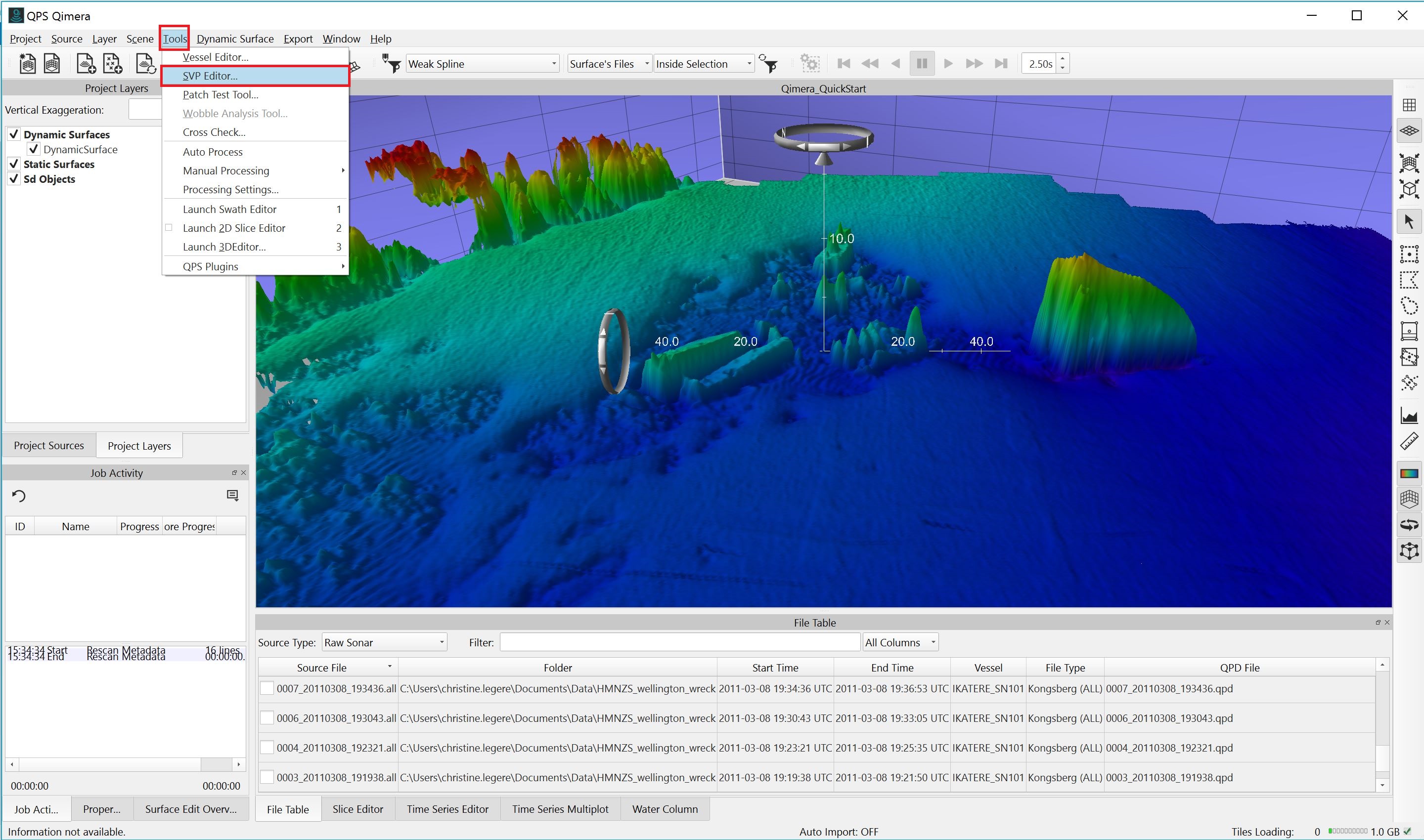
Edit SVP Tool option.
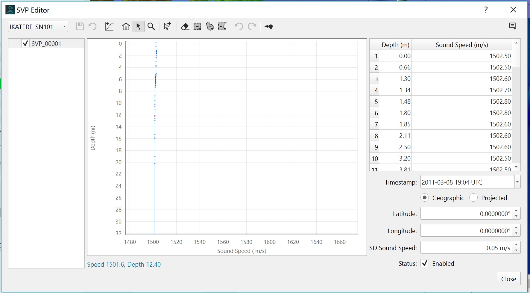
SVP Editor.
When there are multiple Sound Velocity files in your project, you can choose how they are used during processing in the Processing Settings Editor. To access the Processing Settings Editor, select the file or files that you want to apply specific settings to and click on the Processing Settings Button 
Edit Processing Settings.
Select the Sound Velocity tab to review the options for Sound Velocity strategy and prioritization. Make any necessary changes and click OK.
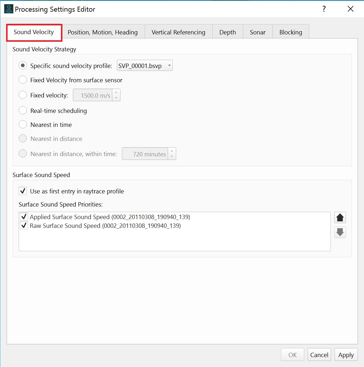
Sound Velocity Processing Settings.
Once this is done, Qimera will mark all affected files as needing processing, indicated by the
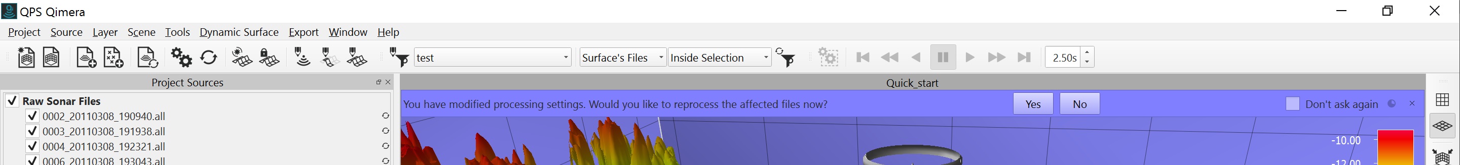
Prompt to reprocess affected files.
Add & Apply Tide Information
Qimera supports a variety of tide formats directly (click here for a list of all supported tide formats); alternatively, an ASCII file with tide information can also be imported and configured. Supported tide formats and ASCII Tide can be added to Qimera by going to the Source menu and select Add Tide File.
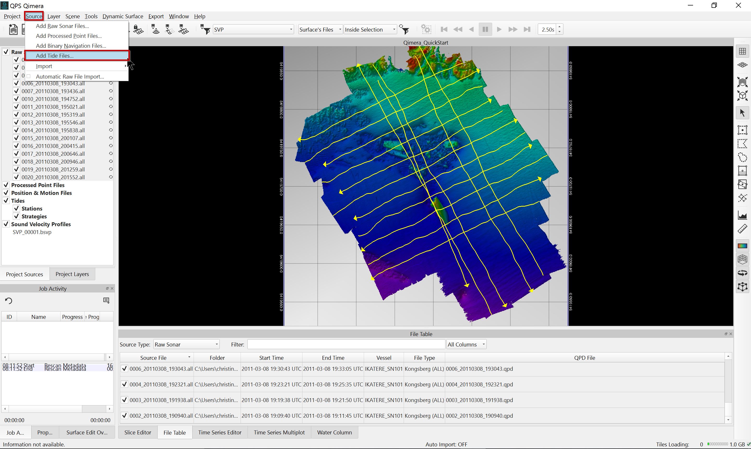
Adding Tide information to Qimera.
Once the tide information has been added to the project it will be listed in the Project Sources Window under Tide Files (1). Adding Tide information will mark all affected files as needing processing (2), indicated by the
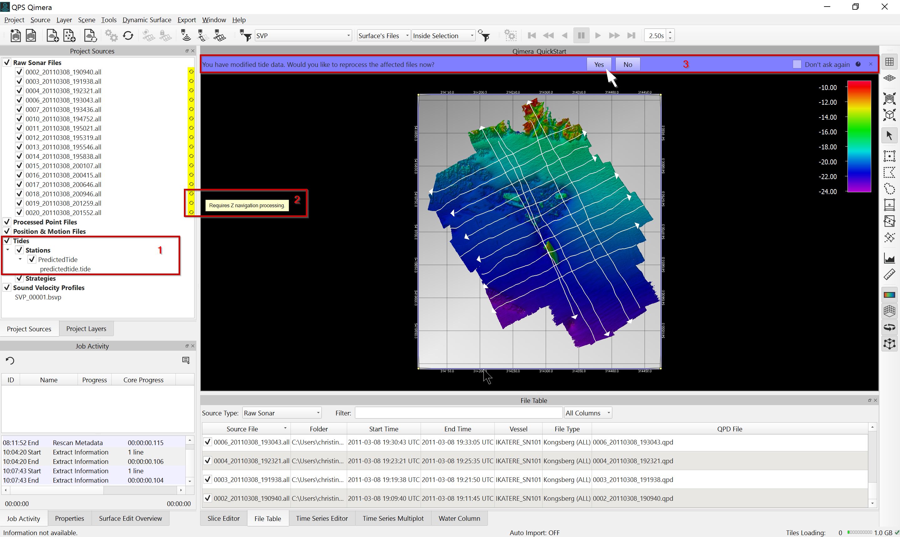
Tide file in Project Sources and subsequent changes/prompts.
After the new information is integrated in all of the affected files, any Dynamic Surfaces utilizing those files will automatically update.
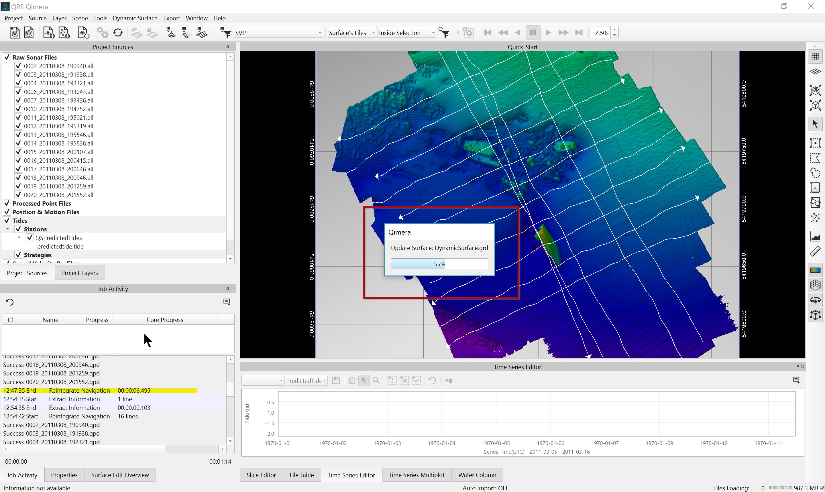
Reintegration of navigation complete; Dynamic Surface updates.
Add & Apply Other Navigation Sources
Other Binary Navigation sources (SBET or POSMV) can be added and used for vertical referencing and/or position/motion/heading. These files can be added to Qimera by going to the Source menu and selecting Add Binary Navigation Files.
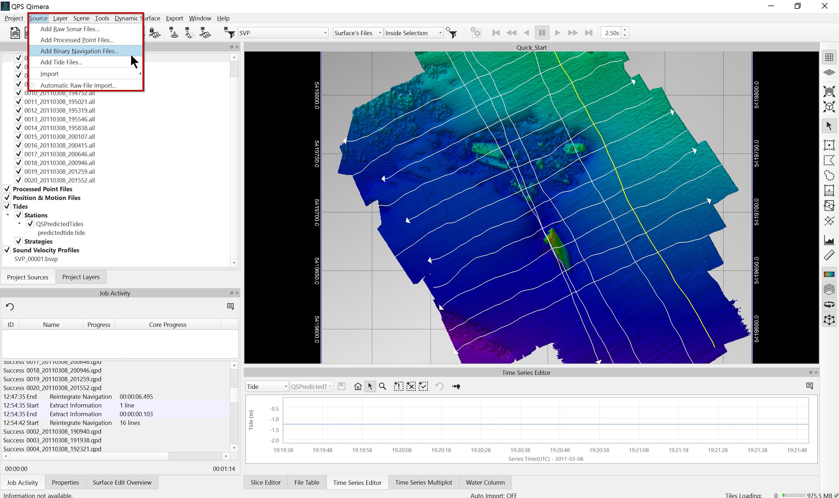
Adding Binary Navigation Files to Qimera.
Once the Binary Navigation information has been added to the project it will be listed in the Project Sources Window under Position & Motion Files. Adding Binary Navigation information will mark all affected files as needing processing, indicated by the
When there are multiple vertical referencing or position/motion/heading sources in your project, you can choose how they are used during processing in the Processing Settings Editor. To access the Processing Settings Editor, click on the Processing Settings Button
Select the Vertical Referencing tab to review the options for Vertical Referencing Method. Importing binary navigation for heighting will change the vertical referencing method to GNSS/GPS and the newly imported information will be set as the top priority item in the list of vertical referencing source streams.
Select the Position, Motion, Heading tab to review the Source Priorities for these three attributes. Newly imported data is always promoted to be the top priority source.
Importing Binary Navigation, Vertical Referencing Method
For more information on the navigation configuration dialog when adding Binary Navigation Files, click here. For a howto on adding Binary Navigation Files, click here. For more information on setting the Vertical Referencing method, click here; a howto on Vertical Referencing can be found here.
Step 8 – Edit Bathymetry
Editing of bathymetry can be accomplished using Area-Based Manual Point Editing in the 3D Editor or Slice Editor, Swath-Based Manual Point Editing in the Swath Editor, by using Filter Operations (ex. Spline), by using CUBE Filtering, or by using a combination of these methods.
Hotkeys
Widgets
When exploring your bathymetry in Turntable Mode of the main Qimera interface and when working in the 3D Editor, you may find it helpful to turn off the Widgets. In Turntable Mode, the widgets can be turned off using the View Widgets
Area-Based Manual Point Editing: 3D Editor
Prior to doing manual editing, you may find it helpful to change your Depth Layer in the Project Layers Window to Shallow or Deep (1). This will draw your attention to all of the spikes on the top of the surface or bottom of the surface, respectively. Note that any edits you make will flag the QPD points on save, and all depth layers will update on save to reflect those changes.
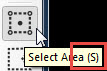
To do Area-Based Manual Point Editing, use the Select Area Mode 


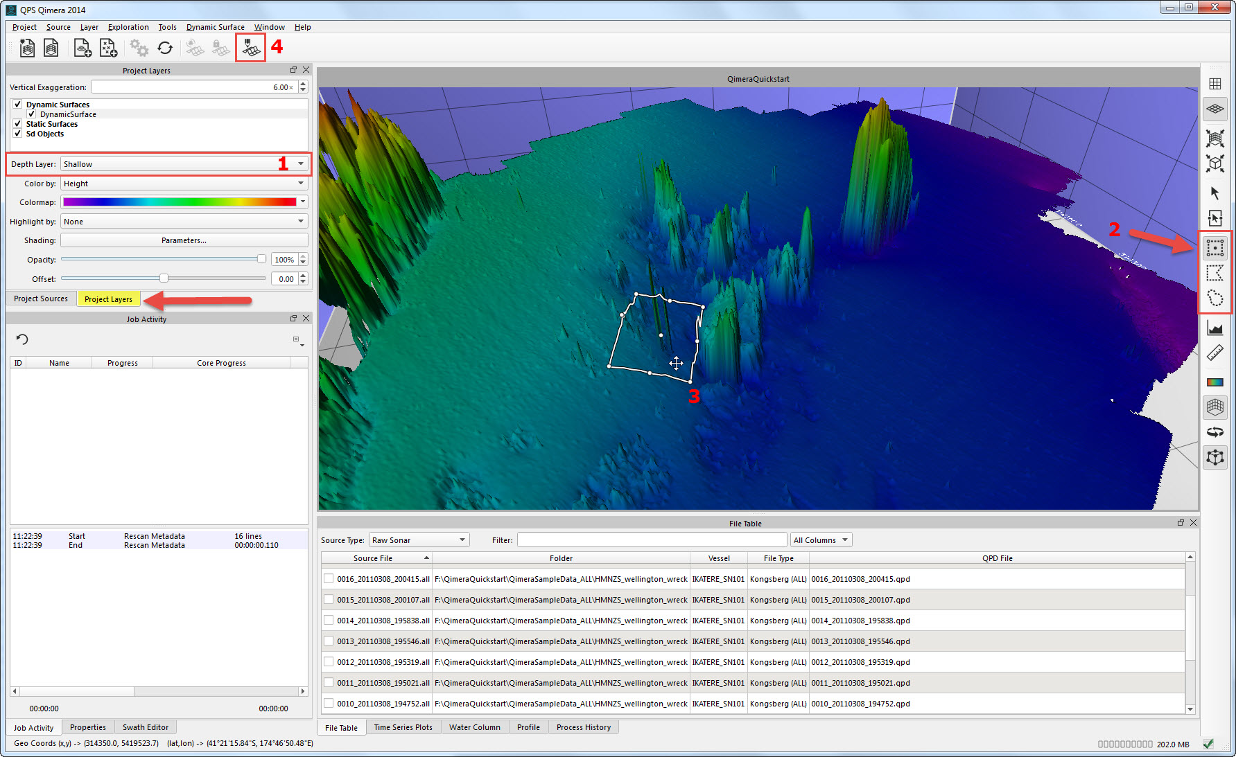
Overview of key Qimera interface elements for Manual Editing.
In the 3D Editor, use Explore Mode 


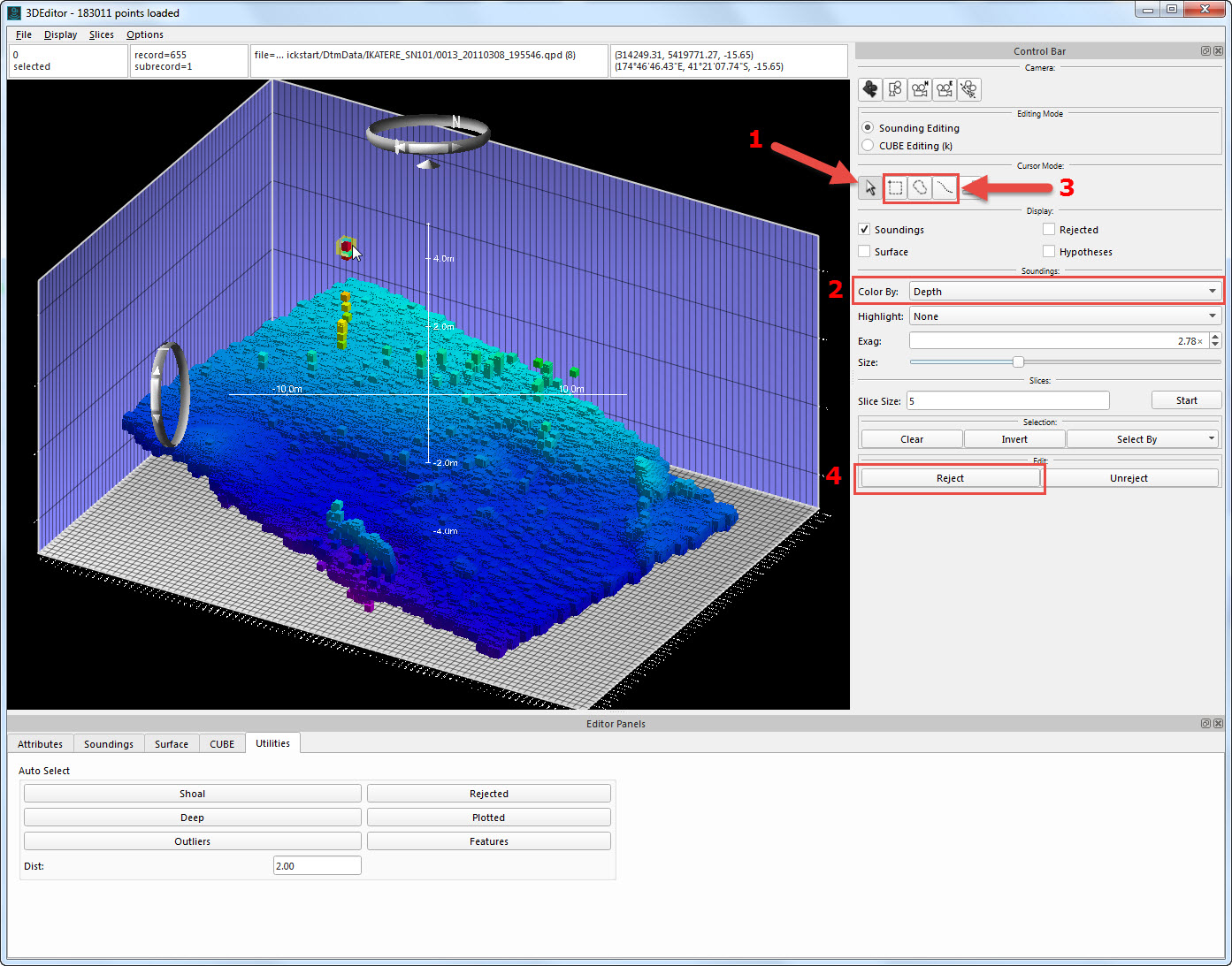
Overview of key 3D Editor interface elements for Manual Editing.
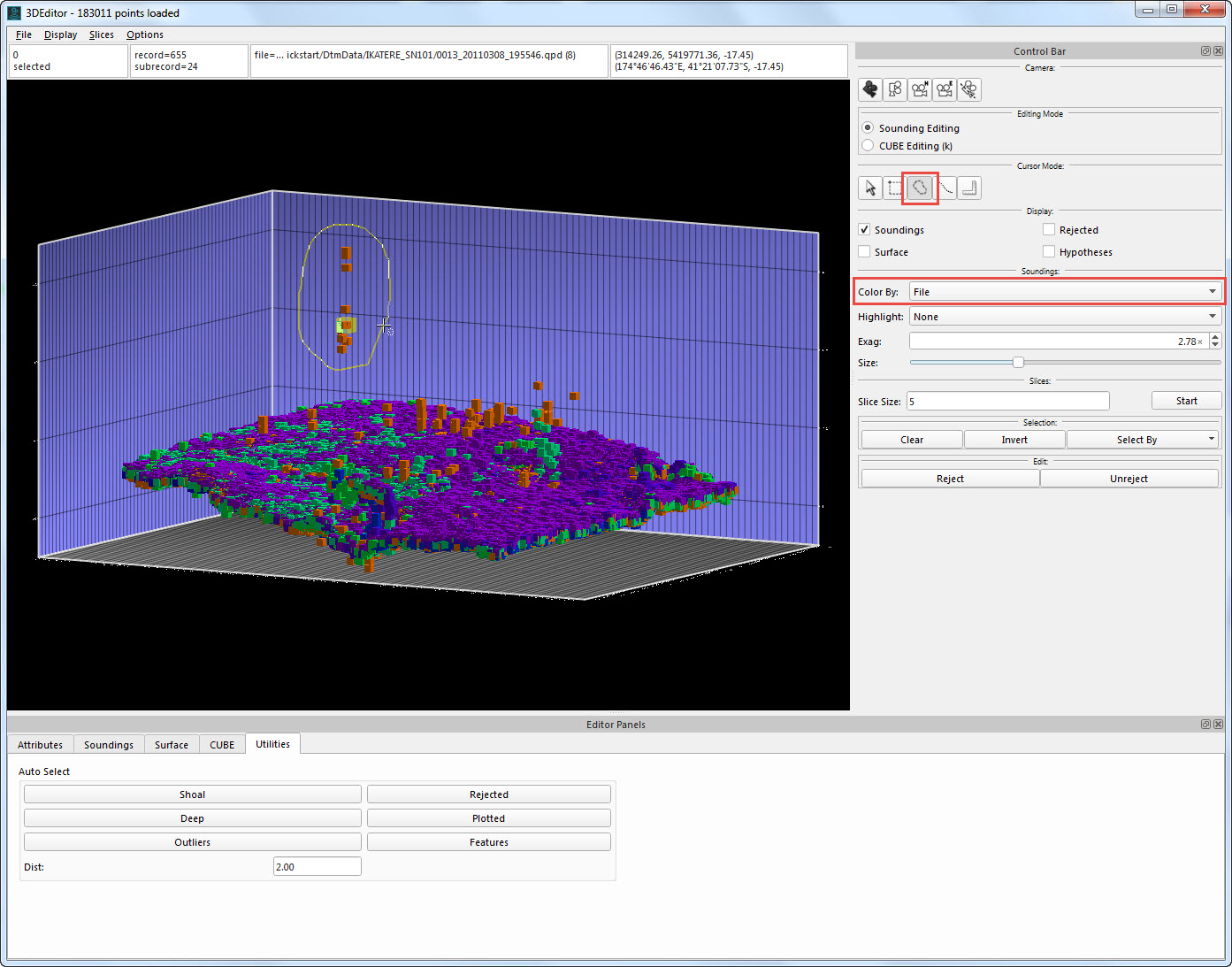
Selection Colored By File; soundings selected for Rejection.
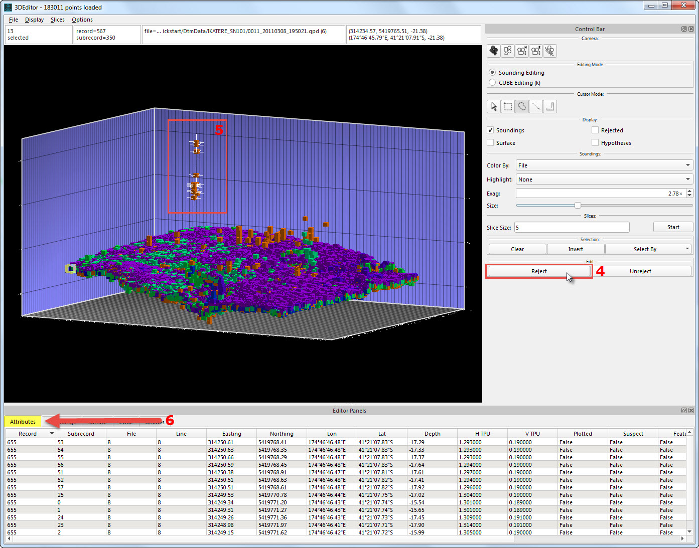
Soundings selected (5); sounding attributes can be viewed in the Attributes tab (6). Click Reject to remove the soundings (4).
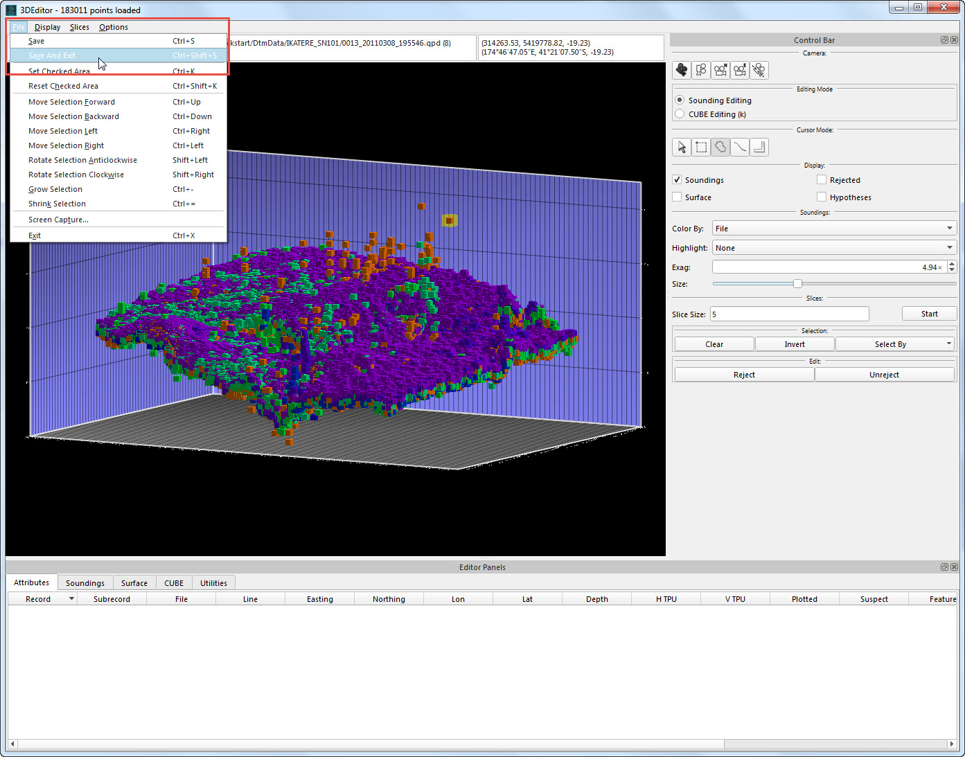
Rejected soundings are removed; Save and Exit to update surface.
Dynamic Surface updated.
3D Editor User Interface
More information on the 3D Editor User Interface can be found here.
Area-Based Manual Point Editing and Filtering: Slice Editor
Please see the How-to Work with Slice Editor for a complete working tutorial. The filtering capability that is outline in the section below can also be applied from the Slice Editor to the data that is currently loaded and visible.
Spline Filtering
Static Surfaces for Filter Check
You may find it useful to create a Shallow Biased Static Surface prior to filtering, to use as a way of comparing the pre- and post- filter results. You can create a Static Surface using the Create Static Surface 
Filtering profiles and advanced application techniques became available in Qimera 1.3. Please see the following references and Howtos for additional information:
Qimera Filter Operation Toolbar
The Spline Filter attempts to fit a surface through noisy multibeam echosounder data and reject all footprints that lie too far from this surface. Spline filtering can be started via the Filter Operation Toolbar or inside the Slice Editor dock, once that has been loaded with points.
To use the Spline Filter, move to the Project Layers and select the Dynamic Surface you would like to filter. Change your Depth Layer in the Project Layers Window to Shallow and preview the surface. This will draw your attention to all of the spikes on the top of the surface. Alternatively, you can set the 'Color by' setting to Standard Deviation. Note that filtering will flag the QPD points, and all depth layers will update after the filter completes to reflect those changes.
A Spline Filter can be applied to the entire selected Dynamic Surface, an area selection (inside or outside) or selected lines within that surface. To limit the area filtered to a line or lines, use Simple Select
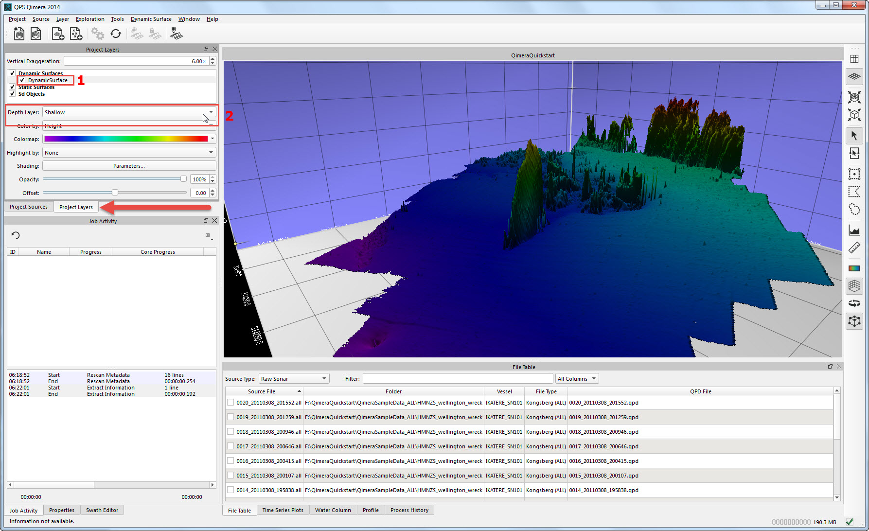
Dynamic Surface selected (1) and Depth Layer set to Shallow.
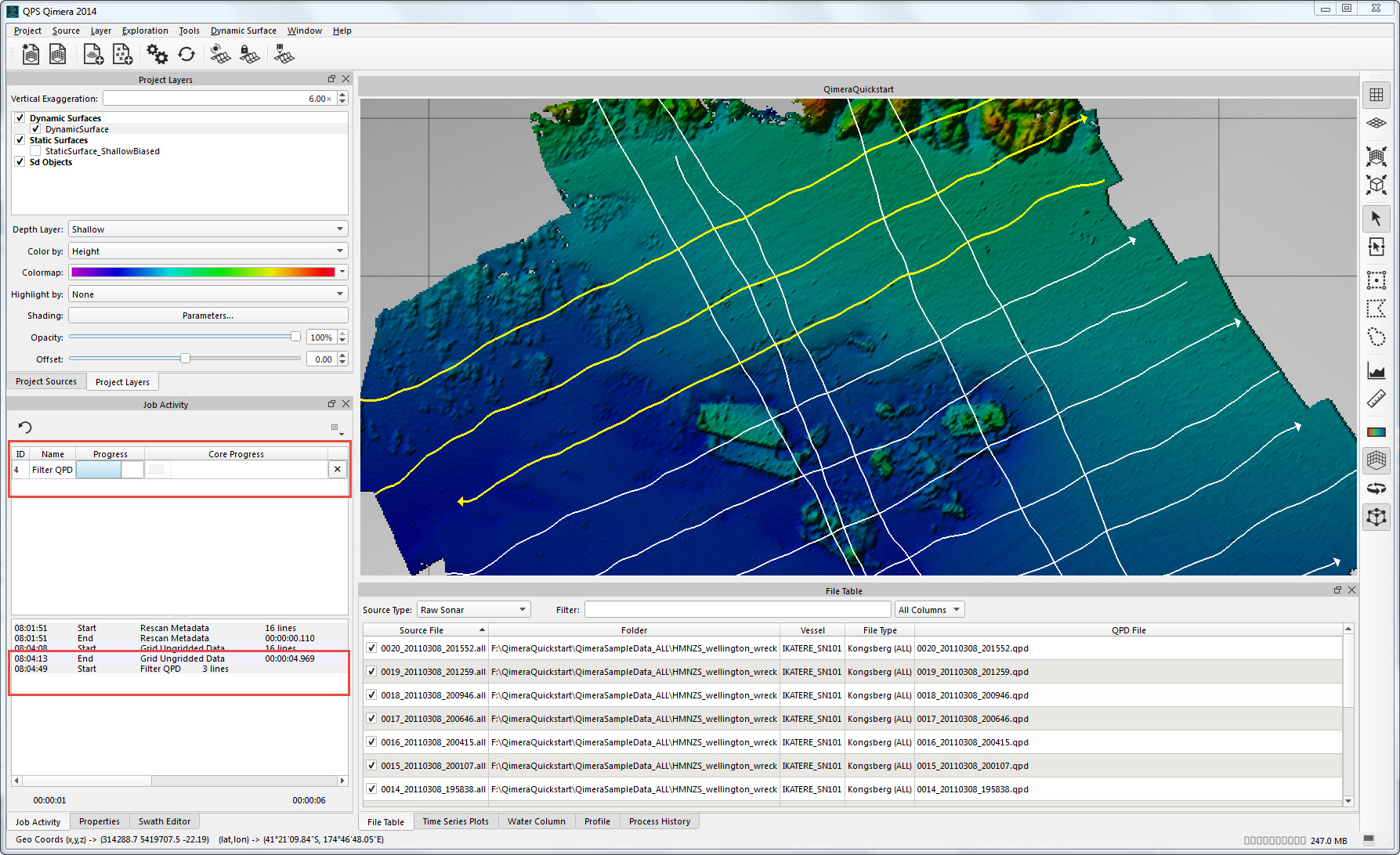
Spline Filter running on selected lines. The Filter progress can be seen in the Job Activity Window.
After the QPDs are filtered, the Dynamic Surface automatically updates.
Review the results of the filter, comparing the new Dynamic Surface to a pre-filter Static Surface if one was created.
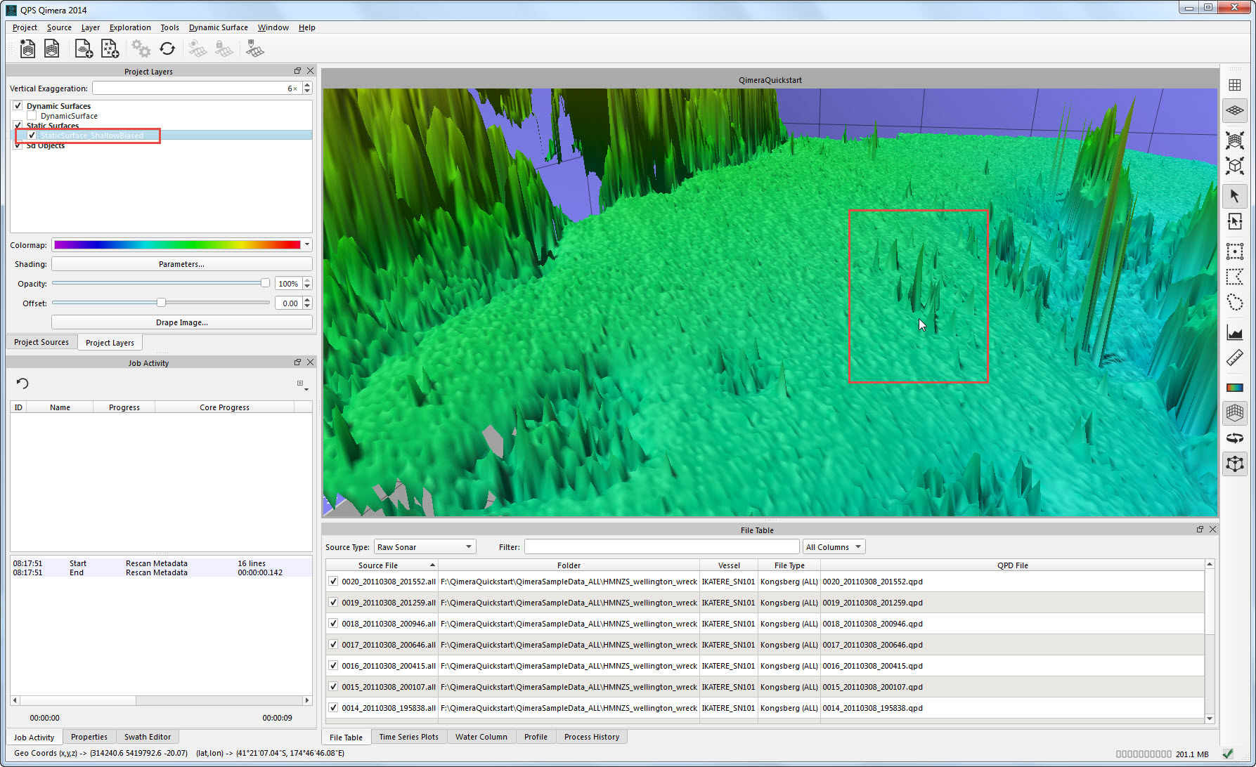
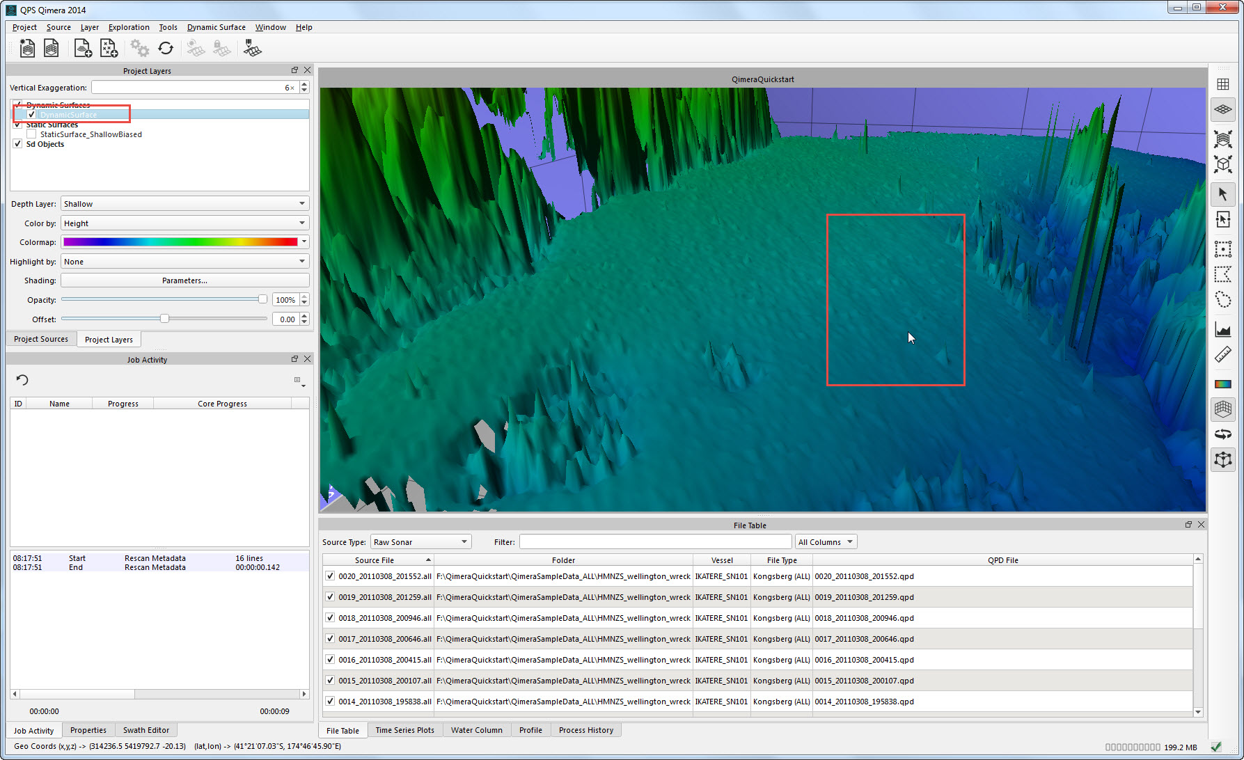
Comparison of a pre-filter Static Surface and a post-filter Dynamic Surface.
Swath-Based Manual Point Editing
Prior to doing manual editing, you may find it helpful to change your Depth Layer in the Project Layers Window to Shallow or Deep (1). This will draw your attention to all of the spikes on the top of the surface or bottom of the surface, respectively. Note that any edits you make will flag the QPD points on save, and all depth layers will update on save to reflect those changes.
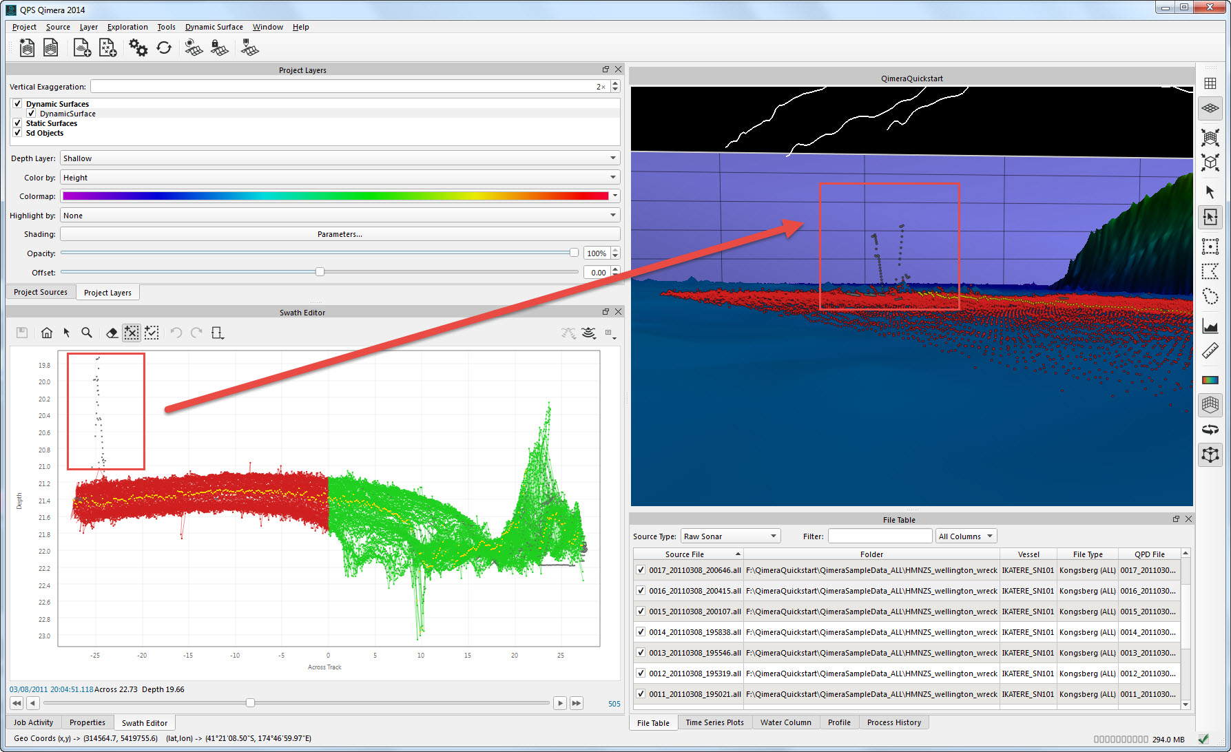
To do Swath-Based Manual Point Editing, select a line for editing either by selecting on the file in the Project Sources Raw Sonar Files tree view (1) or by clicking on one of the tracklines visible in the 4D Scene (the tracklines will need to be checked on in the Project Sources Window). Then, activate the Swath Editor in the Toolbar or press the '1' key. This will load the number of pings defined by the Buffer Width 
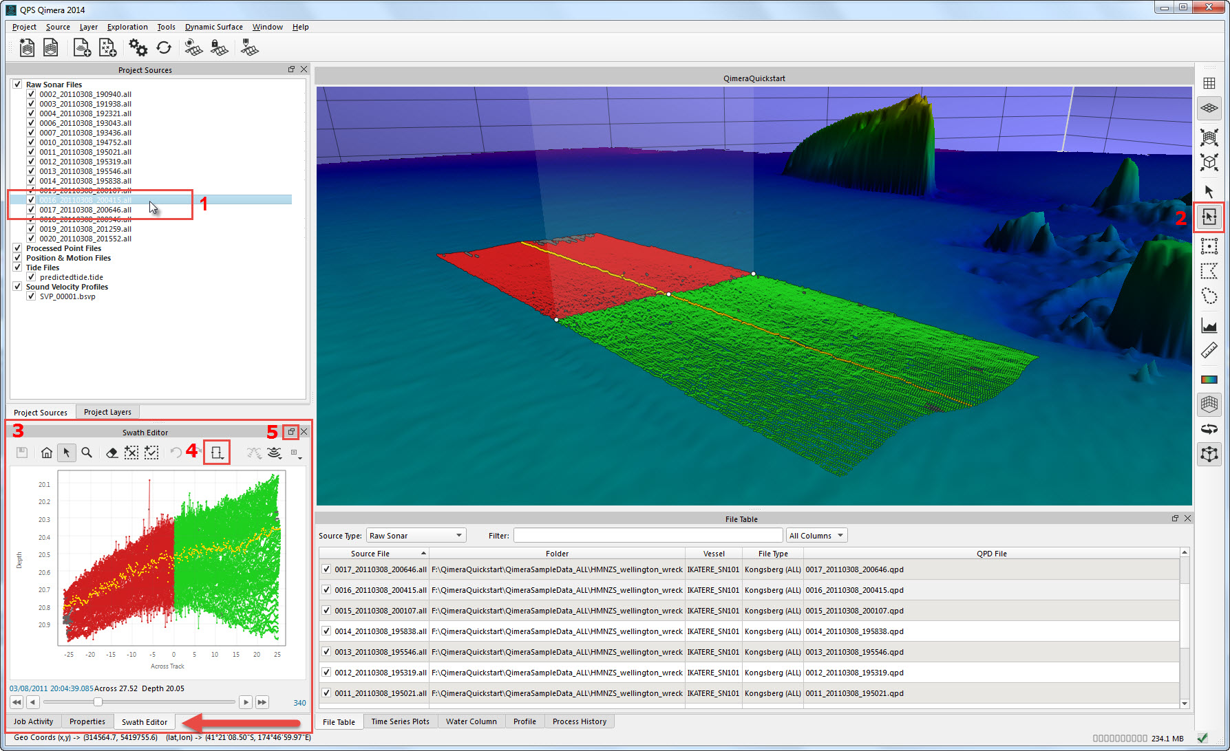
Overview of the Qimera interface when using Swath Editing. Box 1 shows the line selected for editing. Box 2 indicates the Swath Select Mode. Box 3 and the red arrow indicate the position of the Swath Editor Window. Box 4 shows the location of the Buffer Width. Box 5 shows the location of the button used to undock the Swath Editor Window.
In the Swath Editor, use Erase Invalid Mode 

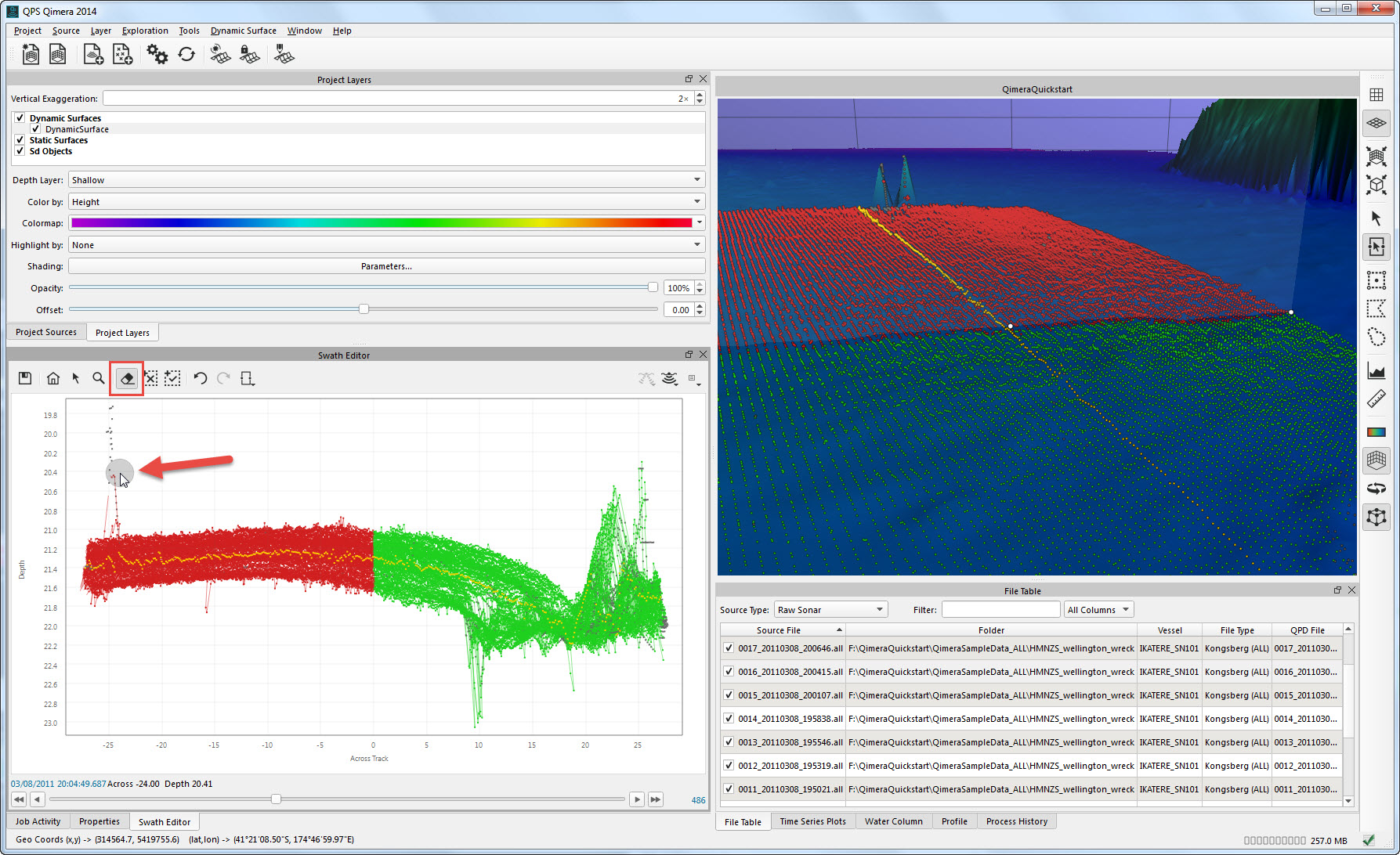
Using Erase Invalid Mode to "erase" and reject soundings.
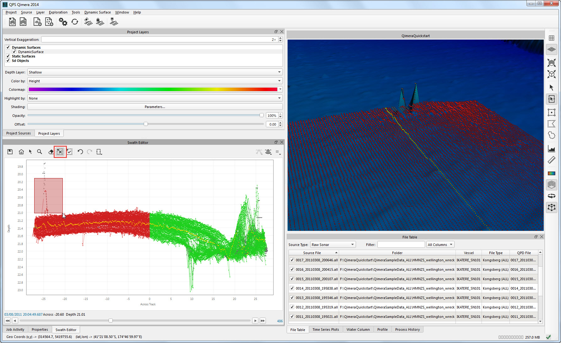
Using Select Invalid Mode to select and reject soundings.
To move along the line, use the Previous Block 


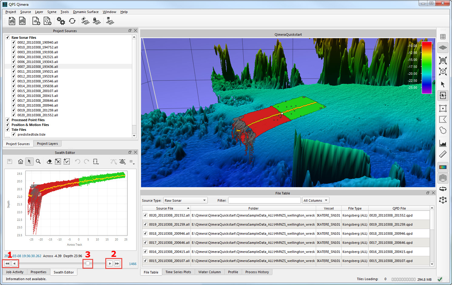
Moving along the line in the Swath Editor can be accomplished using Previous Block/Previous Ping (1), Next Block/Next Ping (2), or the slider (3).
Use the Save Edits 
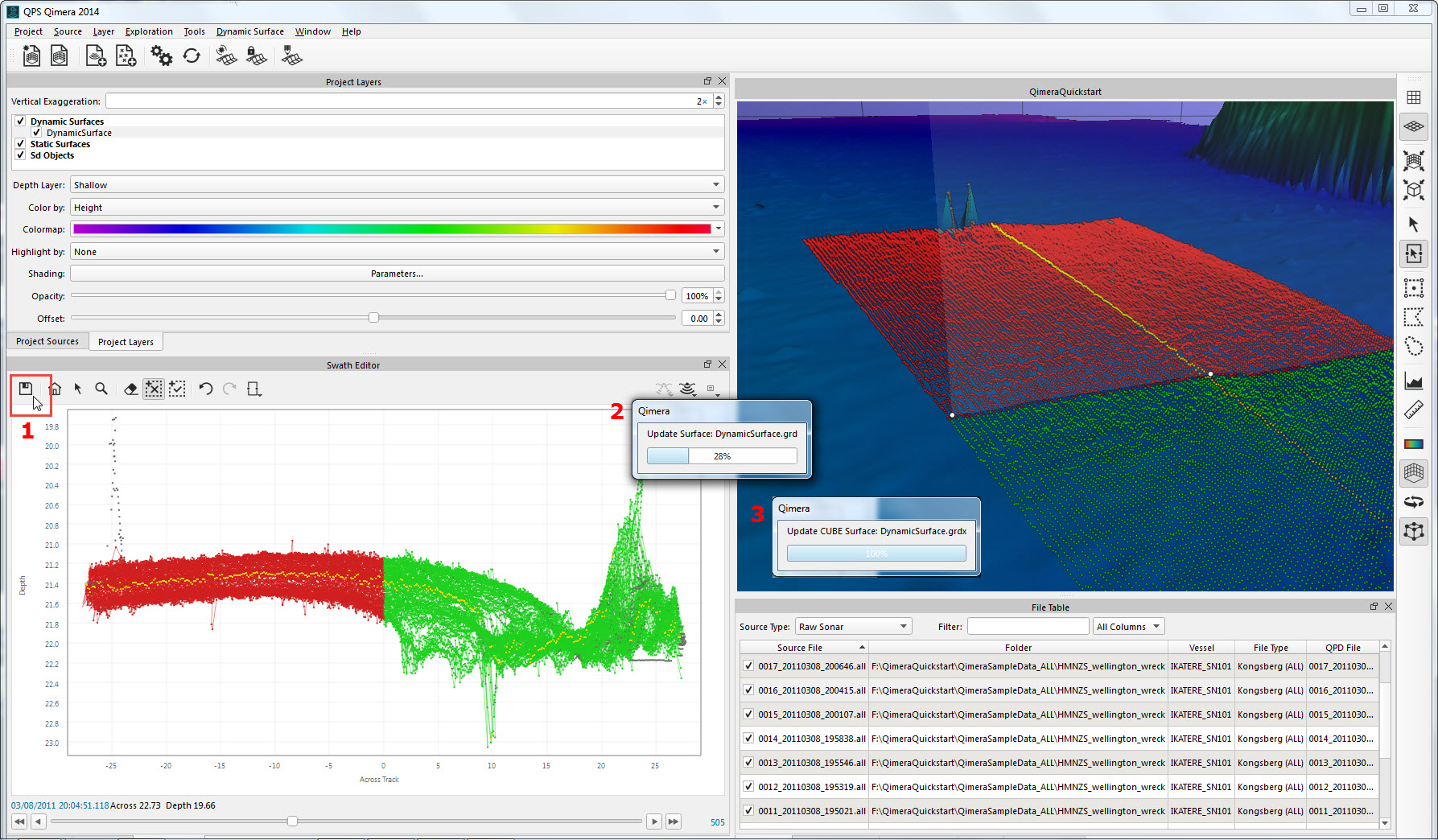
Clicking the Save Edits Button (1) will save changes to the files and force the layers of the Dynamic Surface (including the CUBE Surface, if one was created) to update (2,3).
Saving Changes, Swath Editor
Note that you do not have to save edits if you continue to work on the same line; the edits will be stored as you progress along the line. However if you don't save changes before moving to the next line, the software will prompt you that you have unsaved changes and will force you to save or loose edits at that point.
Grey rejected soundings and updated Dynamic Surface.
Swath Editing
Additional information about cleaning data with the Swath Editor can be found here.
CUBE Editing and Filtering
CUBE Editing results in a clean CUBE surface that can be saved as a BAG (Bathymetric Attributed Grid) or used as a tool for filtering and rejecting all soundings that lie too far from this surface.
To do CUBE Editing, you first must have made the choice to Enable Cube Processing in the Create Dynamic Surface dialog when you built the Dynamic Surface; if you have not, create a new Dynamic Surface and check Enable Cube Processing. Select the Dynamic Surface in the Project Layers Window and change your Depth Layer to CUBE. Change the Color By to Number of Hypothesis; you might find it helpful to edit the colormap to clearly show areas with more then one hypothesis. Review the surface, looking for obvious outliers or areas with multiple hypothesis. Use the Select Area Mode
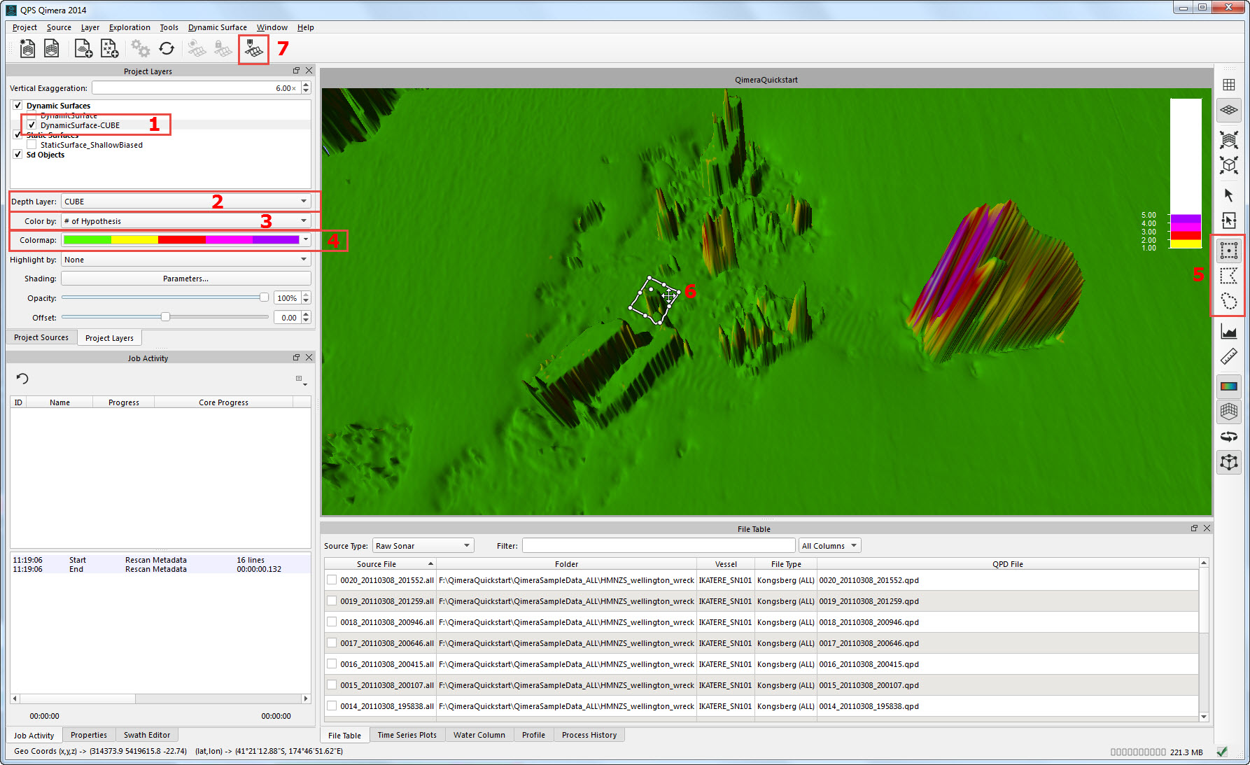
Dynamic Surface with CUBE selected (1) and CUBE Depth Layer selected (2). Color By set to Number of Hypothesis (3) and colormap edited to show areas with more then one hypothesis (4). Explore surface and use a selection mode (5) to select an area (6) with multiple hypotheses. Finally, launch the 3D Editor (7).
In the 3D Editor, check on the Hypothesis Display option (1). Review cells that have multiple hypotheses, comparing the available hypotheses to the soundings to see if the correct hypothesis was chosen (2). If an alternative hypothesis should have been chosen, use CUBE Editing mode (3) and the Select Mode
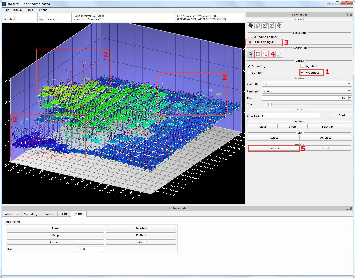
3D Editor showing CUBE hypotheses (1) as well as soundings. Areas with multiple hypotheses (2) should be reviewed. If an alternative hypothesis is more correct, use CUBE Editing Mode (3) and the Select or Area Select Mode to select the alternative hypothesis/hypotheses and click Override (5).
Selected hypotheses in 3D Editor.
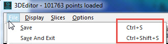
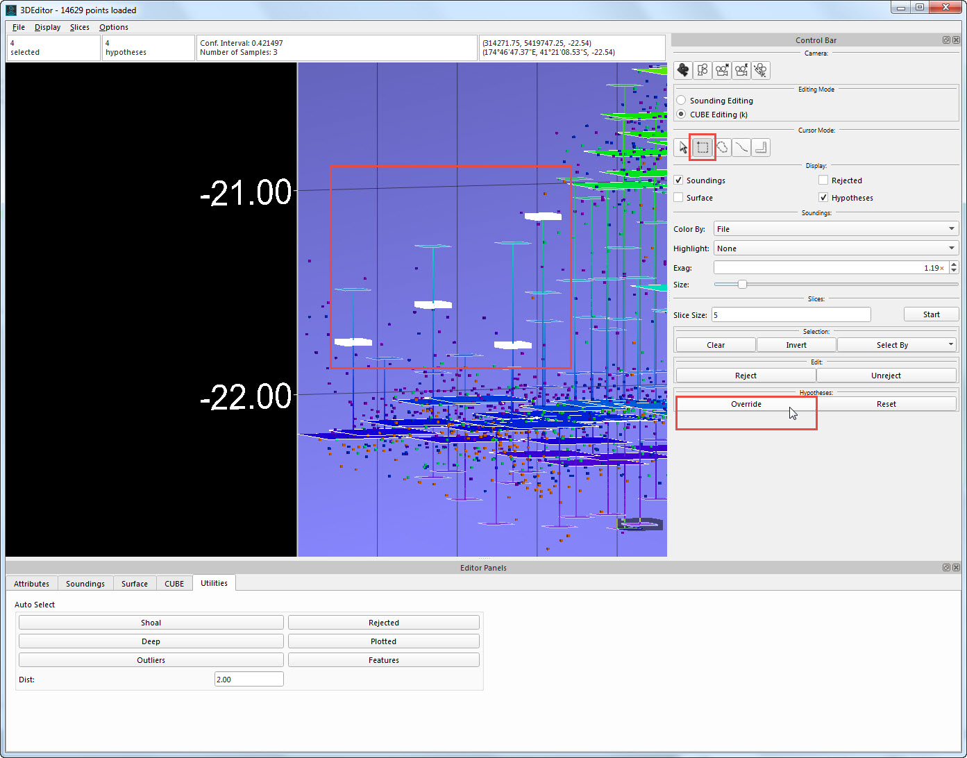
Continue until all necessary hypotheses are updated, then go to the File menu and choose Save and Exit. The Dynamic Surface will update and the 3D Editor will close.
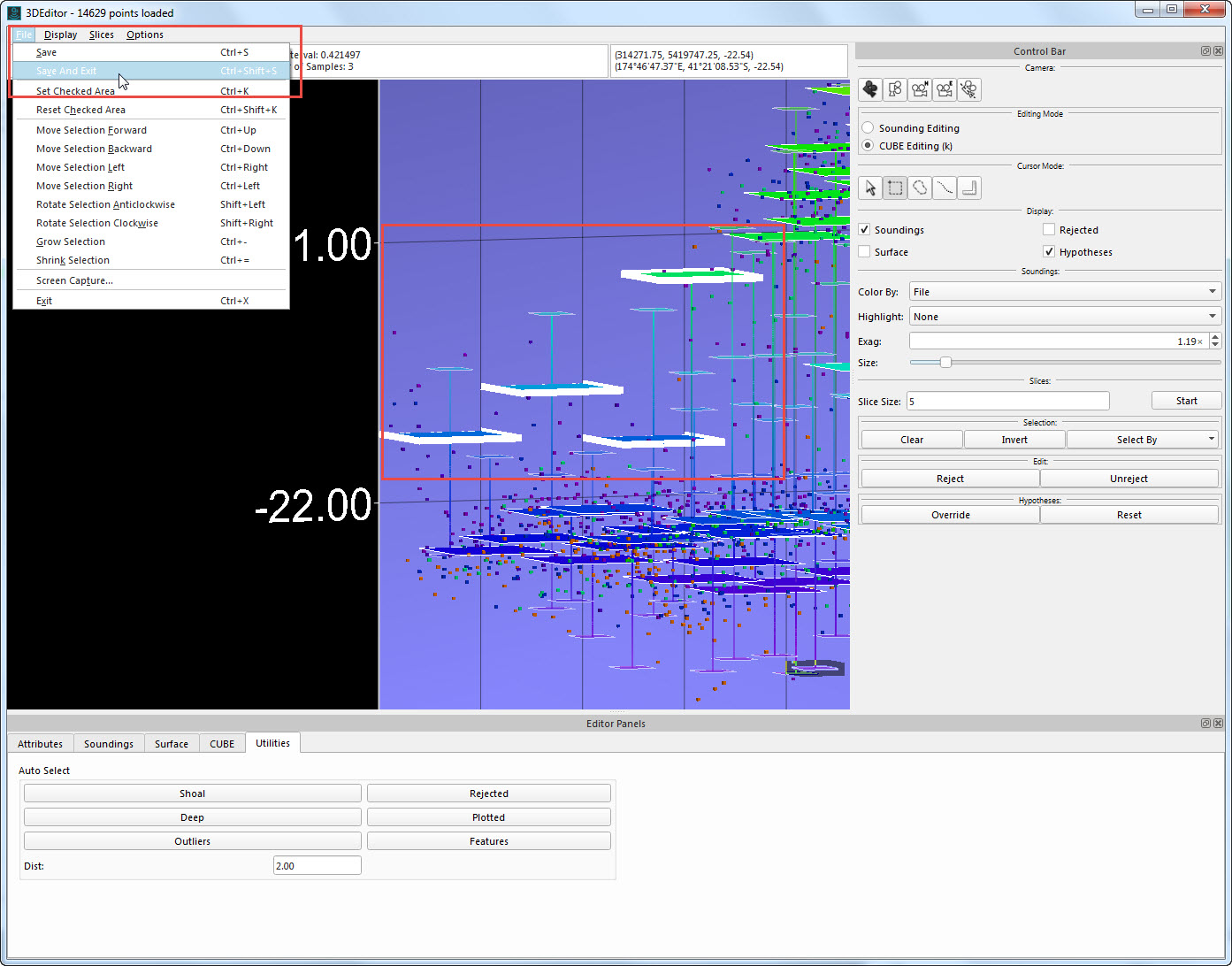
Selected hypotheses after override and location of Save and Exit menu option.
Continue until you have validated the entire CUBE Surface. After you have finished, if your product is a BAG, you only need to export the BAG (see Step 8 - Export Products below). If your product is a clean set of sounding data, you will now want to use the CUBE surface to filter the soundings. The CUBE Filter Soundings option can be run on the entire selected Dynamic Surface or on a selected area of that surface.
Static Surfaces for Filter Check
You may find it useful to create a Shallow Biased Static Surface prior to filtering, to use a way of comparing the pre- and post- filter results. You can create a Static Surface using the Create Static Surface
Select CUBE > Filter Soundings from the Dynamic Surface menu.
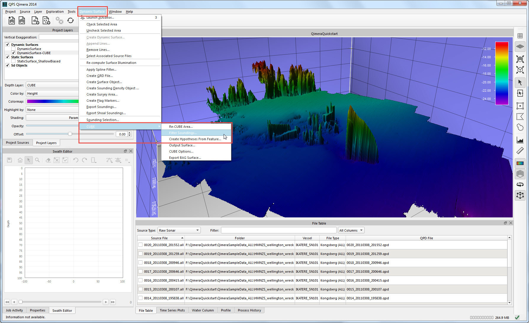
CUBE Filter Soundings menu option.
Set the Filtering Method (1), Vertical range (2), and Scope (3) and then click Filter (4).
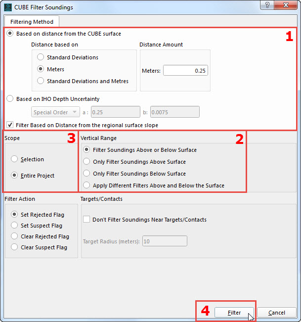
CUBE Filter Soundings Wizard.
The CUBE filter will run, rejecting soundings outside of the threshold you set. The QPD files will update, as will any Dynamic Surfaces that are utilizing the QPD files you just updated. Check your results. Note that the CUBE Depth Layer will show little or no change – check the results of the filter by comparing the Shallow Depth Layer of the Dynamic Surface to the CUBE Layer of the Dynamic Surface (they should now be pretty similar) or to a Shallow Biased Static Surface you created prior to filtering.
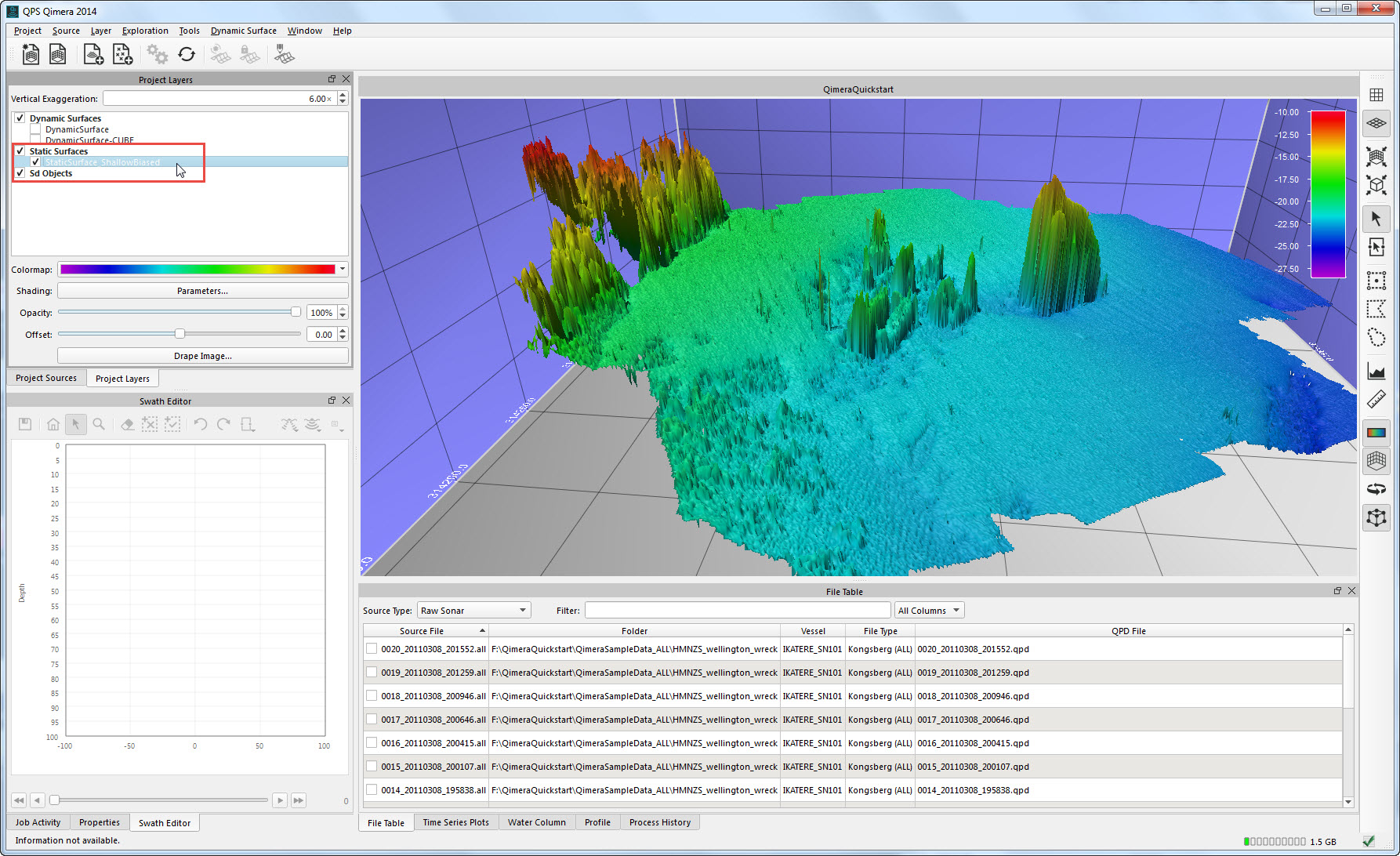
Comparison of a pre-filter Static Surface and a post-filter Dynamic Surface.
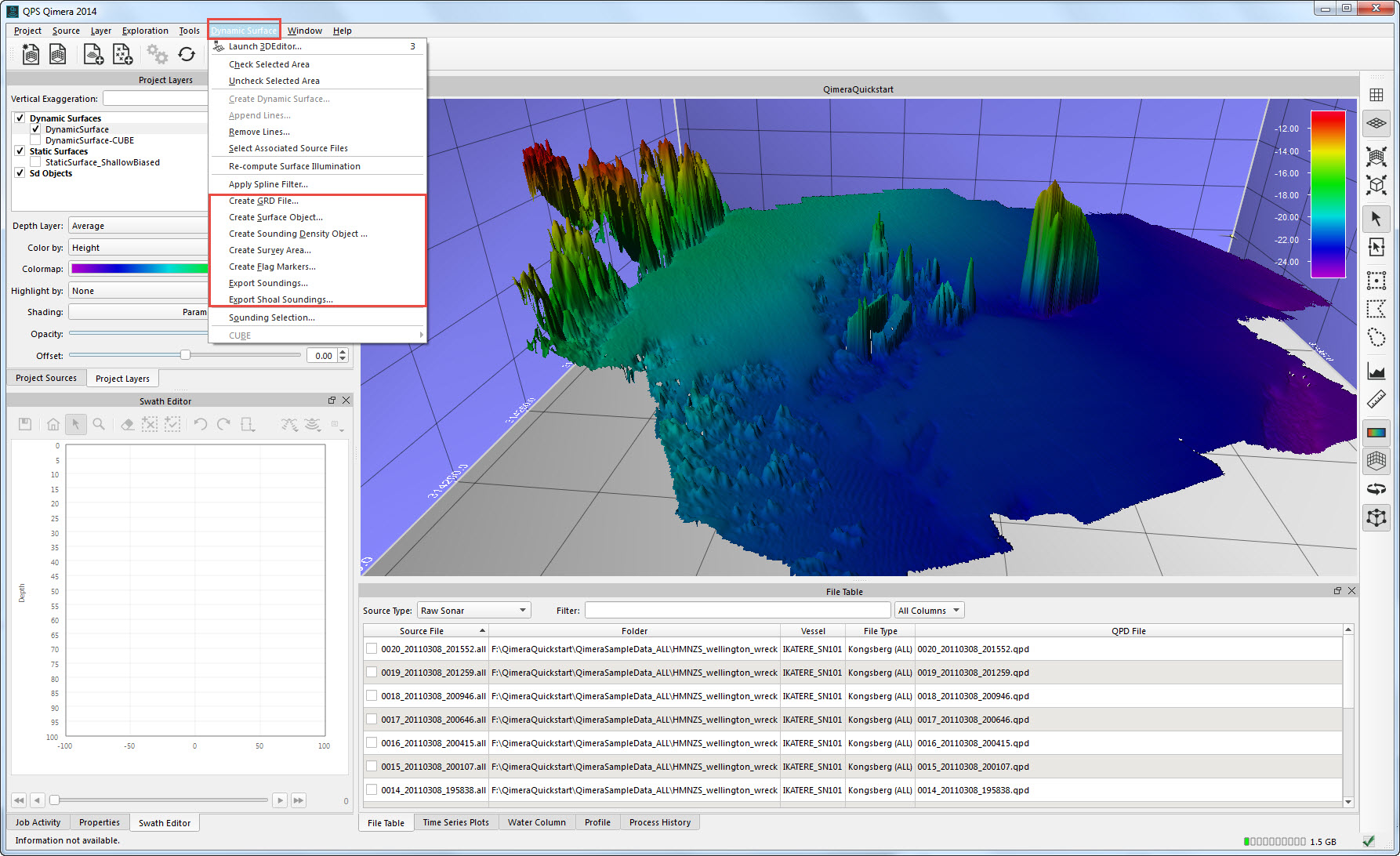
Step 9 – Export Products
Once your processing and editing is complete, you can export products. Exports related to the Dynamic Surface including soundings, https://qpssoftware.atlassian.net/wiki/spaces/qimerakb/pages/43914180, and Fledermaus SD (Snapshot as Static Surface) exports are located under the Dynamic Surface Menu.
Export options related to the Dynamic Surface.
If you Enabled CUBE when you built your Dynamic Surface, additional options will be available under CUBE in the Dynamic Surface Menu.
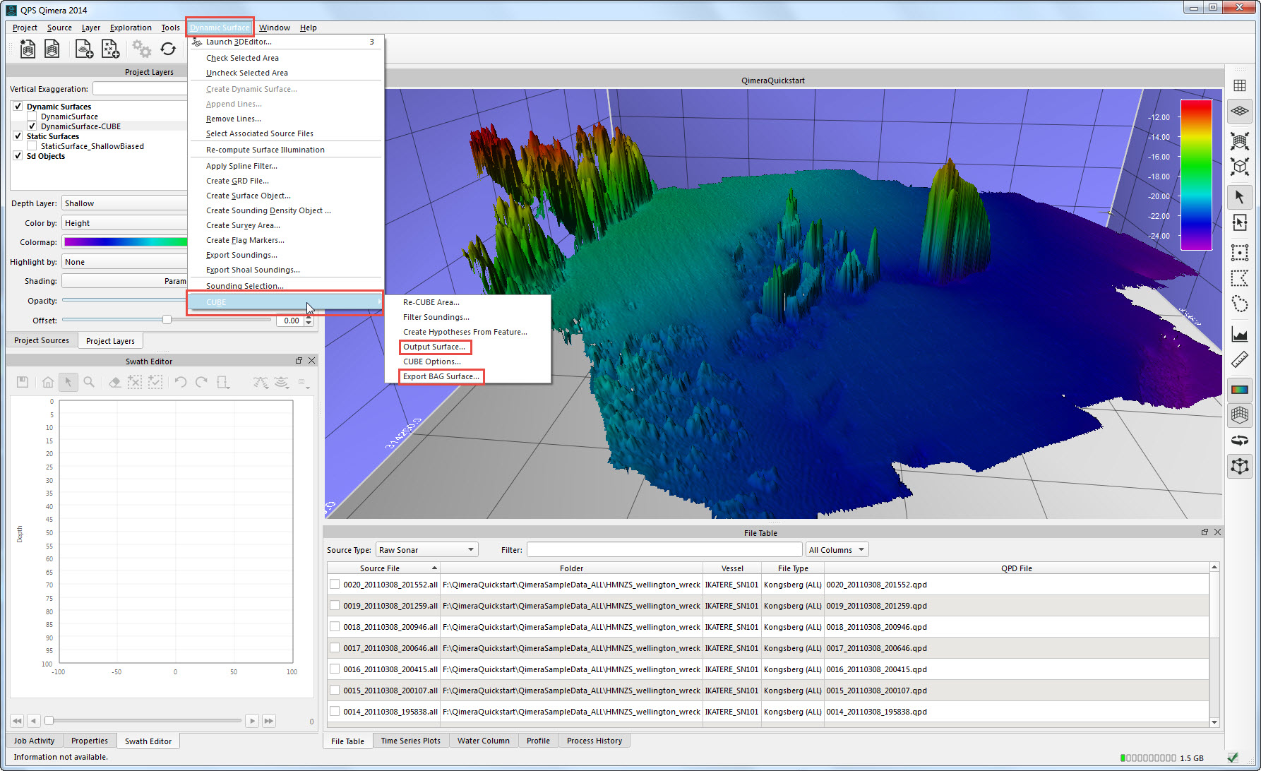
Additional export options related to the CUBE Depth Layer in the Dynamic Surface.
Any surface layer – Dynamic Surface Depth Layers, Static Surfaces, or Fledermaus DTM SD Objects – can be exported to third-party compatible grid formats using Export Surface from the Layer Menu.
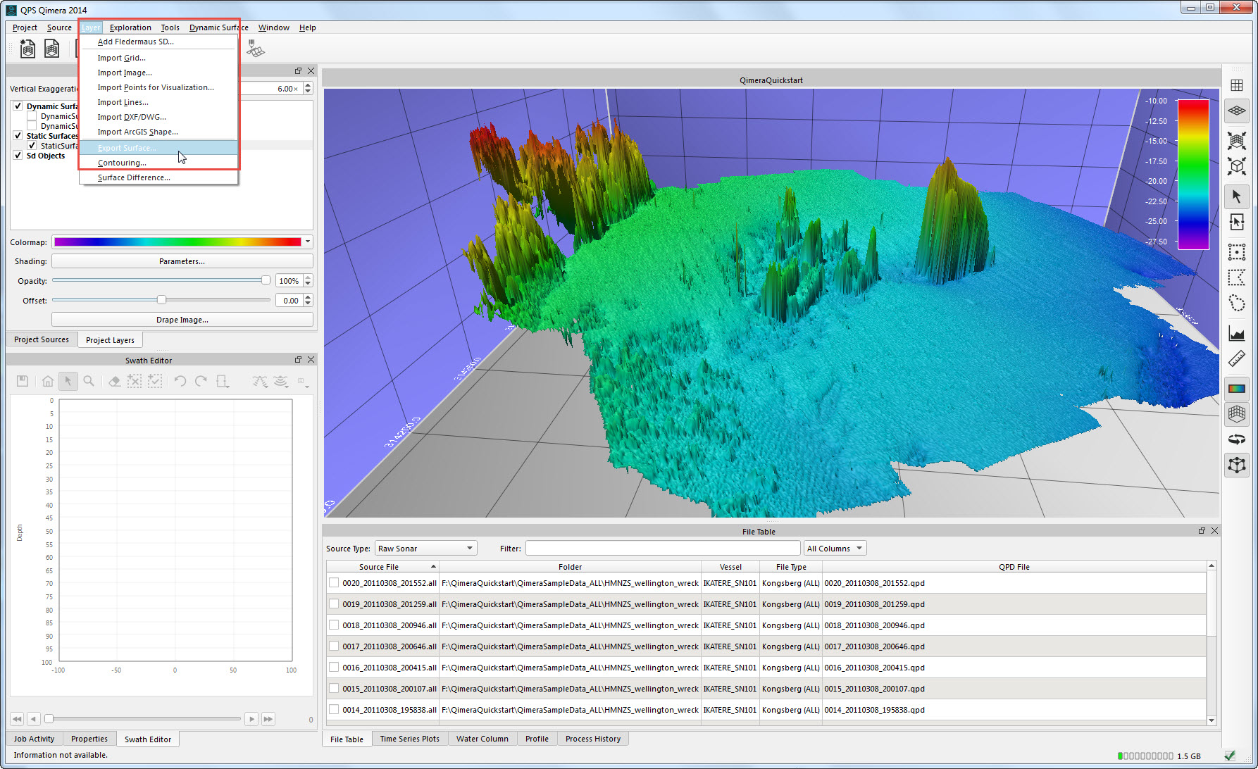
Export Surface option.
Finally, there are additional export options under the Source Menu for exporting processed point information and tracklines.
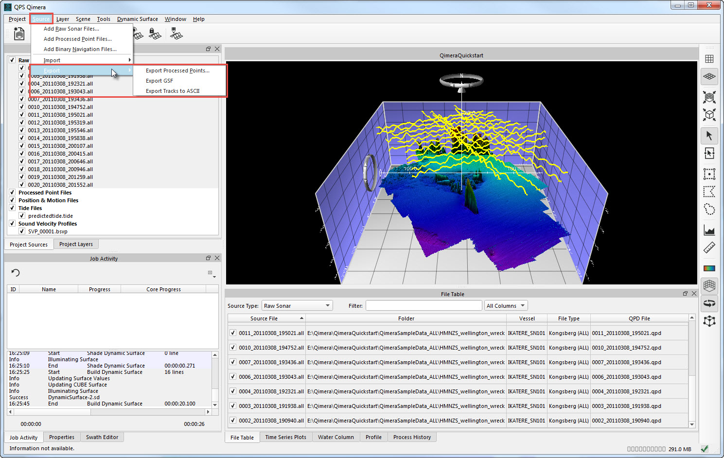
Source export options.
Step 10 – Additional Multibeam-Related Processing
Processing of multibeam backscatter is done using the FMGeocoder Toolbox (FMGT) module of the Fledermaus Suite. For information on migrating processed data from Qimera to FMGT, see How-to Migrate a Qimera Project to FMGT.
Multibeam water column data is processed in the FMMidwater module of the Fledermaus Suite. See the FMMidwater chapter of the Reference Manual for more information.
Step 11 – Surface Analysis
After processing, you may also choose to run surface analysis operations. Operations available in Qimera include Contouring and Surface Difference. These tools can be found under the Layer menu, and can be applied to Dynamic Surfaces, Static Surfaces, and loaded Fledermaus DTM SD objects.

Surface Analysis options.
If you are a Fledermaus Suite user, additional analysis, export, and transfer options are available in the Fledermaus module. You have several options for loading data from Qimera in Fledermaus. A Static Surface generates a DTM SD file in the SD folder of your Qimera project; these files can be loaded to Fledermaus directly by double-clicking on the file in the folder (as long as this option was turned on during installation), dragging and dropping the file in to an open instance of Fledermaus, or by selecting File > Open Data Object/Scene in Fledermaus.
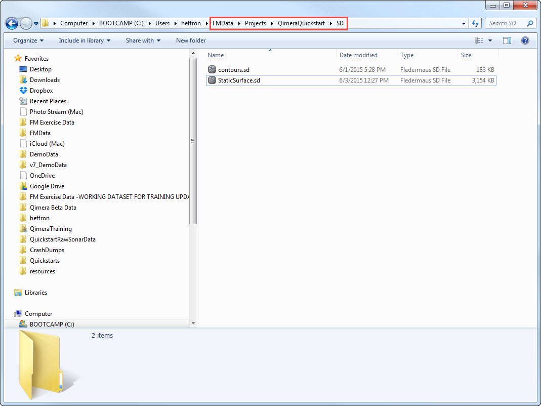
SD files available to be loaded in Fledermaus.
To load a static copy of one of your Dynamic Surface depth layers in Fledermaus, create a Fledermaus DTM SD from your Dynamic Surface using the Snapshot as Static Surface from the Dynamic Surface menu. You can choose to create a Surface Object for a selected area or the entire surface. To create a surface object for the entire area, simply select the Dynamic Surface and Depth Layer of interest in the Project Layers Window prior to selecting Create Surface Object. To create a surface object for a selected area, select the Dynamic Surface and Depth Layer of interest and then use the Select Area Mode
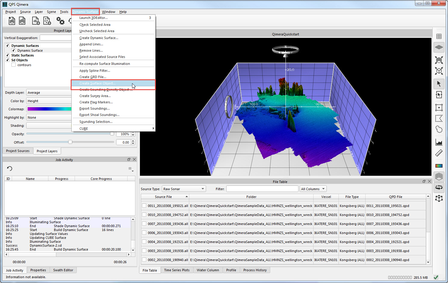
Creating a Surface Object (DTM SD) for Fledermaus.
If you would like to see all available Project Layers of your Qimera project in Fledermaus, the easiest option is to save all of the information to a Fledermaus Scene. Select Save as Fledermaus Scene from the Scene menu. In the Save Scene Options dialog box check on the layer groups you are interested in, then click OK. The scene will save in the SD folder of your Qimera Project with the name Scene_#####.scene. Double-click on the scene icon to launch Fledermaus and load the scene (as long as this option was turned on during installation), or alternatively launch Fledermaus and select File > Open Data Object/Scene and browse to the scene in your Qimera SD folder.
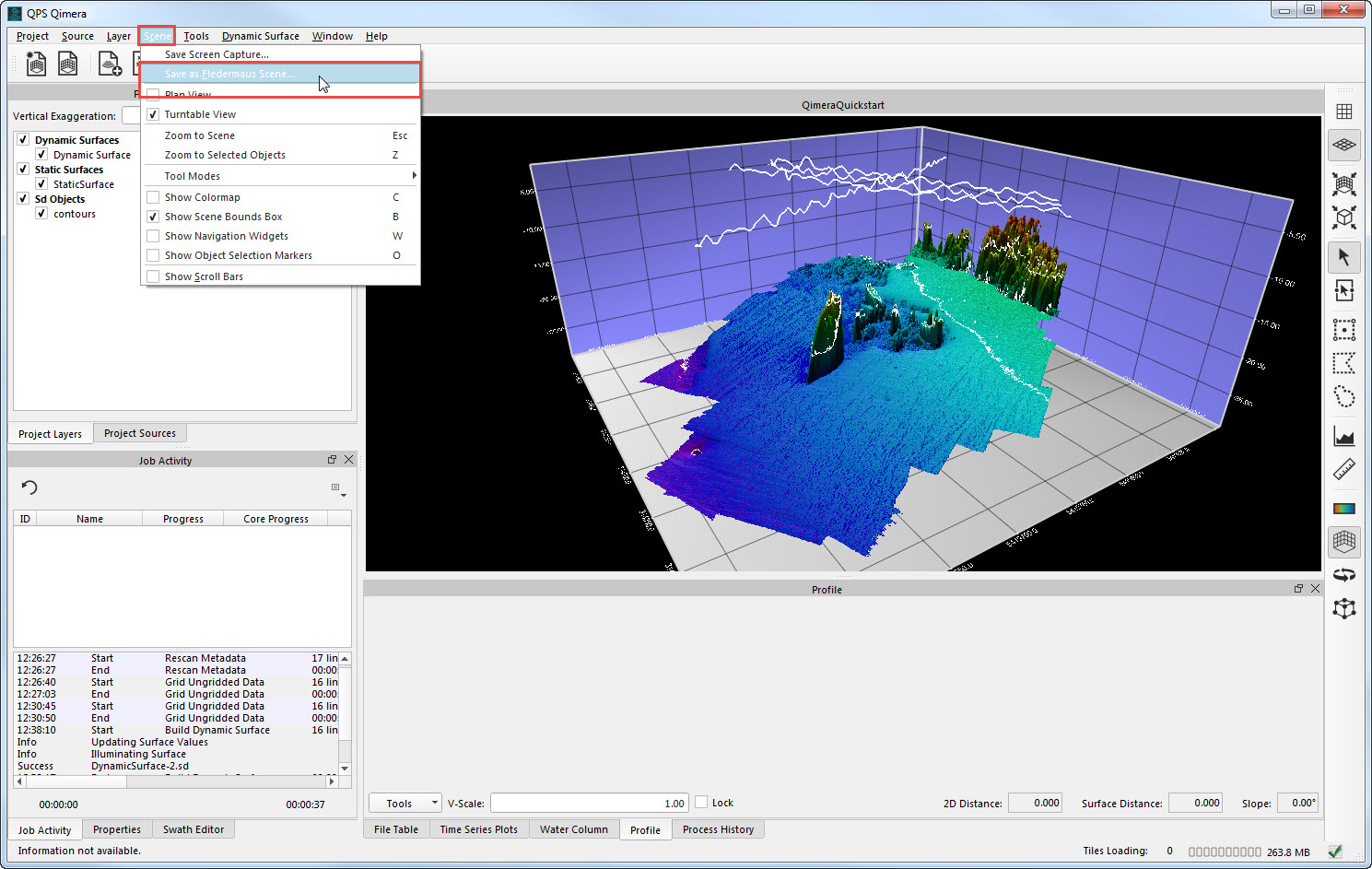
Saving Qimera layers as a Fledermaus Scene.
Loading Qimera-generated Surfaces in Fledermaus
As noted above, Static Surfaces and SD object generated in Qimera can be loaded to Fledermaus for further analysis. Currently, Dynamic Surfaces cannot be loaded in Fledermaus; in the current releases of Fledermaus, leaving the Dynamic Surfaces option checked in the Save Scene Options (image above) will trigger a warning in Fledermaus: "Problem reading file: some or all of the file may not load". This will not prevent other layers from loading correctly. The functionality to load Dynamic Surfaces will be available in a future release of Fledermaus.