How-to - Adjust Bias for Uncalibrated Data

This how-to outlines how to adjust for bias' in uncalibrated data. 

Step-by-step

Step 1: Import files

Create a new project and import two files, one for each head of one survey line, made with a dual headed system. Since the adjustment for bias is between two heads, the data from each head must be evaluated individually. 

Ideally the data would be from an area with a flat seafloor. Additionally, be sure to uncheck the tick-box next to 'Merge into single file' if using the paired files import. 

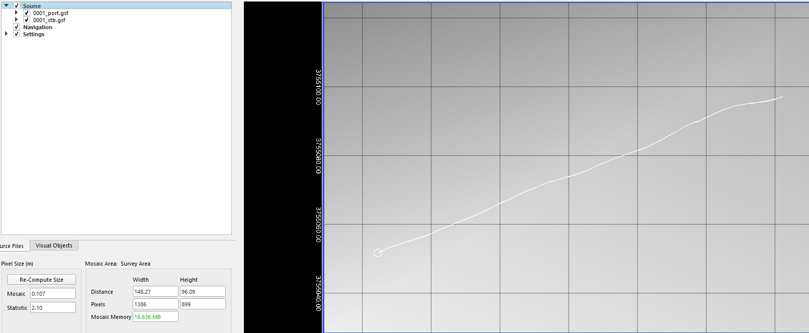
One way to easily obtain one file for each head is to bring your line into Qimera, and export the line as two gsf's, one for each head (So you will export data twice).

Step 2: Create Mosaics

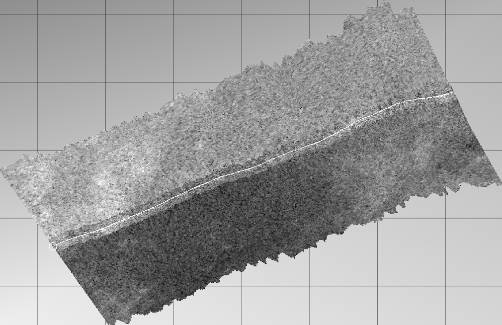
Create a separate mosaic for each head, and rename accordingly. As you can see in the image below, there is an offset between the two heads.

Step 3: Mean Backscatter Value 

Selecting one mosaic at a time, determine the value of the peak of the histogram in the bottom window for each mosaic, and compare the two values. There are two ways to do this: 

Option one: Hover over the peak of the histogram with your mouse. The value will be returned in the middle of the window below the histogram. 

Starboard Head:

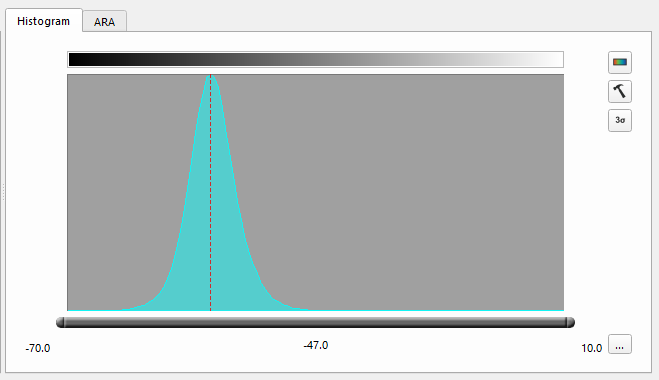
Port Head:

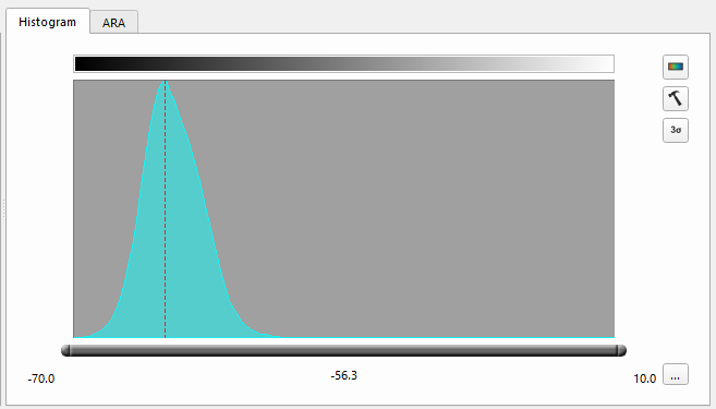
For example, in the images above we see that the starboard head has a peak of -47.0 dB while the port head had a peak of -56.3. So there is a difference of 9.3 dB between them. This difference value is what you will need in the next step.

Option two: Navigate to the messages tab, and using the selection tool,  select along the mosaic of both heads. At each click the messages window will update with information on the selected ping: 

The value that is needed for the bias is the mean backscatter value and the difference from the last selection. This option is more accurate when more selections are used. For example the pings selected in the above image shows that the mean difference is 7.5 dB, or 7.8 dB as a difference of the means. Meanwhile with more subsequent selections and comparisons, the mean difference is 9.77 dB and the difference of the means is 10.07 dB. These values are much closer to the value obtained using the option one method shown above, and are therefore more likely to be closer to the real bias value. 

Step 4: Set Processing Parameters

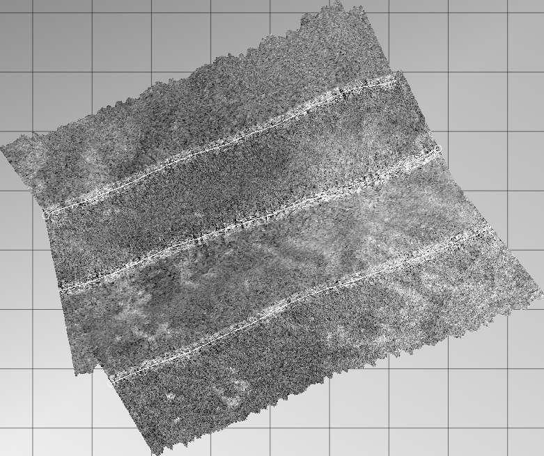
Create a new project, bringing in all full lines of data (if you haven't made one already). Create a mosaic of all lines, to compare before and after applying a bias. 

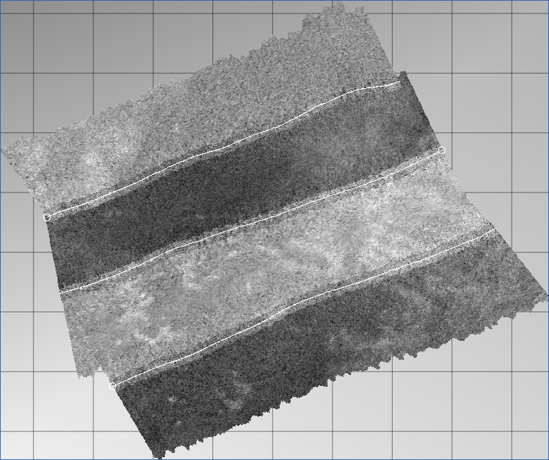
Next, create a new settings profile (Settings>Add Processing Settings), and name it appropriately. In the adjust tab of the settings editor (Settings>Processing Parameters> Edit New Settings Profile), under the backscatter range header, you can input the difference found in step 2 in one of the head bias prompts. 

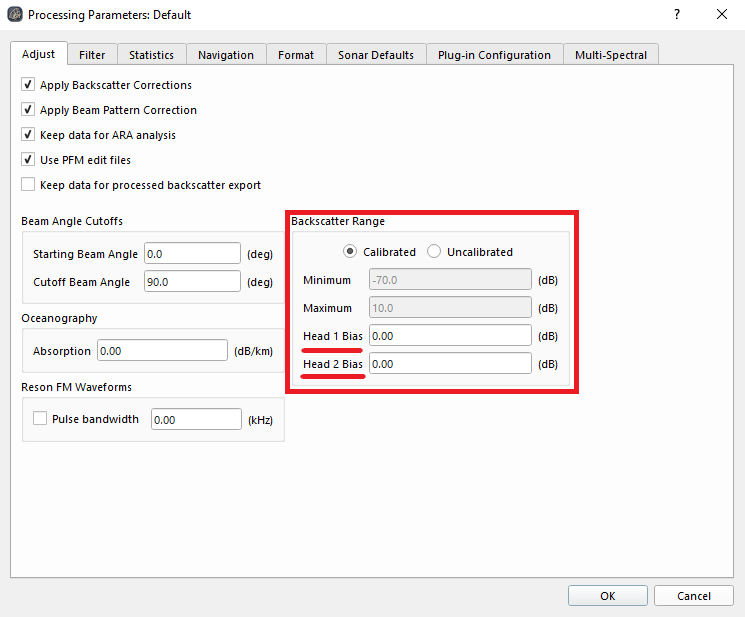
For example, the difference found from the data used in step 2 was 9.3, with the Starboard head having the higher value. Thus a value of 9.3 can be inputted into the head 1 bias option, or a value of -9.3 can be inputted into the head 2 bias option. It just depends on which head you would like to stay as it is, and which head you would like to change to match the other. 

Save these changes, and close the settings editor. 

Step 5: Apply Processing Parameters

Apply your new settings profile to all of your files by right clicking the "Source" item at the root of the Source Files tree and choose "Set Settings". Then select the settings profile you just created. 

Your files will need to be reprocessed, and then any difference between the two heads should be fixed. Create a new mosaic to view the results.