Imagery Visualization Classes
This small family of data types involves those that deal with the visualization of 2D imagery data and the variety of methods that they can be visualized and represented in the 3D virtual world of Fledermaus. The class types include the GeoImage, Vertical Image (VImage), and Vertical Curtain (VCurtain) classes.
GeoImage Class

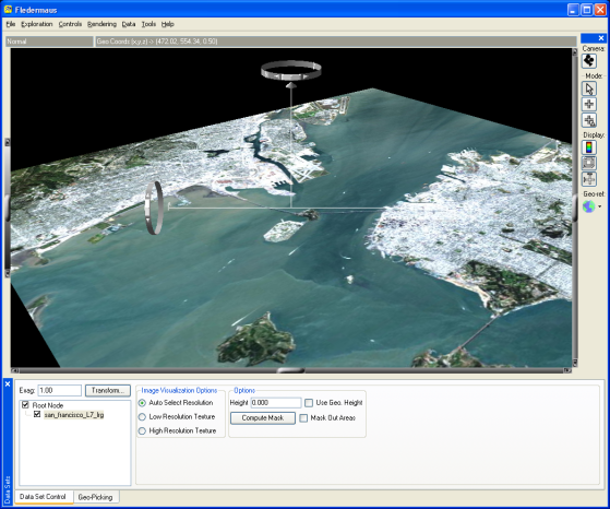
Figure 1 28 - Sample GeoImage
Imagery has many uses within the Fledermaus visualization system and is commonly draped on related surfaces. It is often very useful to be able to bring 2D imagery into the 3D scene to complement the 3D data currently loaded. For example, one might have a bathymetric map showing the depths of a lake or river channel and want to bring in a satellite image of the region. The 2D image can be added to the scene as a geo-image object and properly geo-referenced within the scene (see Figure 128). To add the image, select the Import > Import Image File menu option and select an image file with the standard file selection dialog box.

Figure 1 29- Geo-Image Controls
GeoImage objects can also dynamically interact with the scene via the controls in Figure 129. The Image Visualization Options control what is displayed for the GeoImage when in explore mode. If Low Resolution Texture is selected, a low-resolution version of the image is displayed and the High Resolution Texture option causes the actual pixels from the image to be displayed at all times. If the Auto Select Resolution toggle is enabled, the ShiftScapeTM rendering engine will automatically decide when to use high-resolution or low-resolution textures.
By default, 2D images are assigned a height of 0.0 (sea level) but the height can be interactively controlled by entering a value in the Height field.
Tools Menu

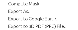
Figure 1.30 Tools Menu
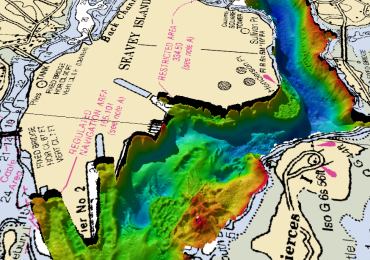
One method of combining DTMs and GeoImages into a single scene is to mask the image. This is done by using surfaces in the scene to "knock holes" in the imagery over the location where its data resides, which makes the the imagery visible through the surface data. To perform this operation, click the Tools -> Compute Mask menu item and select the Mask Out Areas toggle. An example of a masked image is given in Figure 1.31.
The Tools -> Export As... option exports the GeoImage to a GeoTIFF file. Export to Google Earth... will export files for viewing in Google Earth. The Export to 3D PDF (PRC) File... option will save the image to a 3D PDF file for viewing in compatible 3D PDF file viewers such as Adobe Acrobat Reader. Optionally, a PRC (Product Representation Compact) file may be saved.

Figure 1 31 - Example of Masking a GeoImage
Vertical Image Class

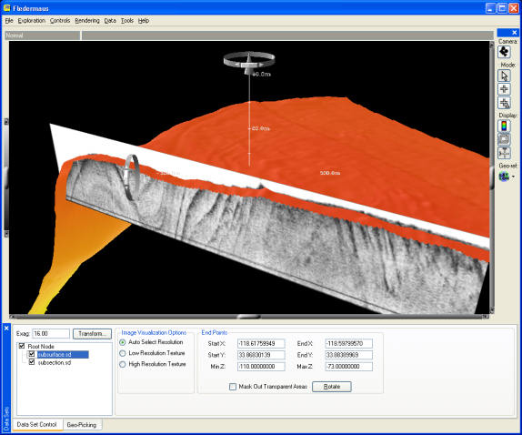
Figure 1 32 - Sample Vertical Image with a DTM
The Vertical Image (VImage) class is a close sibling of the GeoImage class. It provides many of the same features with the exception that this surface is perpendicular to the XY plane. As an example this could be an image of a parameter in the water column, or a seismic profile of the sub-surface (see Figure 132). The input required is the image in a format supported by the application (such as a tiff image), the coordinates of the left and right-hand edge of the image, and the Z range of the image.
Vertical Image Controls
The procedure for adding a vertical image to the scene is similar to that for the GeoImage. Click the File > Import > Import Vertical Image menu option and select an image file with the standard file selector dialog box to add a VImage to the loaded scene. Enter the co-ordinates of the left and right hand edges in the Start X, Start Y, End X, and End Y textfields, and the Z range in the MinZ and Max Z textfields, all shown in Figure 1.32. When moved, the Vimage must be geo-referenced to properly place it in the 3D scene (i.e. the Geo-Reference button must be clicked). Vertical Images can also be created with the mkvimage command line program. Click the Rotate button to rotate the vertical image clockwise by 90 degrees.
The Use Low Resolution Texture, Use High Resolution Texture, and Auto toggles are similar to those controls in the GeoImage class. The Mask Out Area toggle is also similar to the GeoImage class but requires that the source image file contains an alpha channel with white in the areas to mask out.
Vertical Curtain/Seismic Class
The Vertical Curtain (VCurtain) class is similar to the vertical image class with one key difference. In the Vertical Image class the resulting image is still flat, a plane arbitrary orientated perpendicular to the XY plane. In this class the vertical (Z) range of the data is held constant but a geographic location of each column of pixels in the image is specified. Thus the imagery can weave in and out according to the points specified. A good example where this type of class is very useful is in the visualization of processed seismic imagery where the image follows the track of the ship that collected the imagery. Vertical Curtains can be generated through the mkvcurtain command line program.

Figure 1 33 - Vertical Curtain Controls
The controls for the VCurtain class are shown in Figure 133. The Mesh Gap textfield can be used to display a coarser curtain while exploring and the Auto toggles notifies the ShiftScapeTM rendering engine to automatically adjust the mesh gap. The Use Low/High Resolution option will display a low-resolution image while exploring and a high-resolution image when the scene is full drawn. The Use Low Resolution option will always display the low-resolution image and the Use High Resolution option will always display the high-resolution image. With the Auto Select Resolution option enabled, ShiftScapeTM chooses whether to use high or low-resolution textures.
To mask out the black areas of the curtain, click the Compute Mask button and select the Mask Out Areas check box. Note that some VCurtains are generated with a mask so it will not have to be calculated.
You can get help using the mkvcurtain command by running it in fmcommand with the -h option. The basic help is:
INFO: Usage:  mkvcurtain
                 < -in <imageFile> >
                 < -out <sdOutFile> >
                 < -xy <xyFileName> > | < <-start x y> <-end x y> >
                 < -zrange zmin zmax >
                 < -ocoordsys <OutputCoordinateSystemName> >
                 [ -mode <simple | distance | geomatch> ]
                 [ -h ]
   This program takes as input an image file that represents data in the vertical
(z) axis such as a seismic rendering of a dataset along with a two dimensional path
and z-range. It then places the vertical slice in the fledermaus scene according to
the supplied info. The x and y values must be in the units of the output cordinate
system. The -mode option controls how the coordinates of the xy file
are mapped for each column of pixels. The default simple mode evenly distributes the
coordinates along the image. The distance mode properly distributes the points based
on the relative distances between points. The xy file can also have an optional third
parameter which forces the coordinates to be fixed to a particular pixel column
with the remaining points evenly distributed. If this information is provided then
the geomatch mode must be used.
To help explain how the mode option works, assume we have an image to be visualized as a vertical curtain and that image has a width of 1000 pixels. To geo position the vertical curtain we need to provide a file of x and y coordinates along with a z-range. The most basic way to position your vertical curtain is to supply a file of 1000 x, y coordinates, one position for each column of pixels in the input image. However, to simplify things you can provide less points and still properly geo-reference the image. For example, if the vertical image path is a straight line you need only two x y coordinates. The mkvcurtain problem provides 3 modes to help. The “simple” mode just takes however many input (x, y ) points you provide sets the 1st column of pixels to be at the 1st position given and the last coordinate to the last column of pixels and evenly distributes the other positions along the image. The “distance” mode examines the distance between each point and distributes the positions to pixel columns accordingly. So for example if you gave the xy file three points and the distance between the 1st and 2nd point was 50% of the distance between the 2nd and 3rd point. Then the in resulting curtain the 2 point would be positioned at column 333 of the 1000 column wide image and the remaining points computed accordingly. When the geo-match option is specified and you include a 3rd value in the input xy file you can more precisely control the matching. For example say you provide a xy file like:
400000.0 500000.0 0
400050.0 500000.0 500
400200.0 500000.0 1000
The 3rd parameter is which column of pixels the given position should be mapped to. In this case the 2nd point will be the position of the 500th pixel column with the remaining points distributed accordingly even through the distance between the 2nd two points is much greater. Given this same file with the “distance” option used the 2nd coordinate would be given to 250th pixel position instead. Note you can specify -1 as the position of the last point and the system will automatically substitute the position of the final column of pixels.
Return to: Reference Manual
