
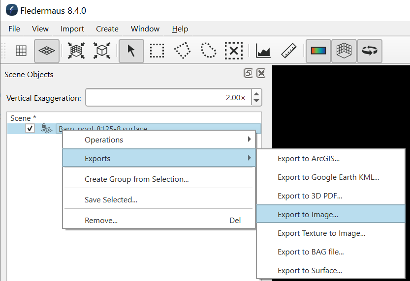
This technical note convers some important details related to exporting and rendering surface data into an image and saving the results. If you have a surface object and you want to turn it into a properly geo-referenced image file, the best way to do this is through right clicking the surface object and selecting the Exports > Export to Image... option as shown below.
This will bring up a dialog with a number of options to control the export. There are two different methods that are used to turn a surface into a saved imagery. One is conversion and the other is rendering and both have an important place and it is important to understanding the differences. The export dialog looks like:
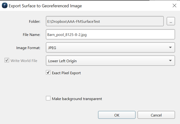
The "Exact Pixel Export" controls which method, conversion or rendering is used. When exact pixel export is on you are getting the conversion method. In this case each cell of the existing surface is turned into an image pixel. The color of the pixel will be the color of the surface you would see when any texture rendering (if present) is turned off. If the surface is 1000 x 500 cells the resulting image will have exactly 1000 x 500 pixels and the geo-referencing will match the edge-to-edge coordinates from the surface. The resulting image may or may not look like how the surface appears on the screen (especially if you have draped imagery on the surface being displayed). The saved imagery is coming from a direct conversion of the data it is not the rendered product as seen on the screen.
On the other hand if you turn off the "Exact Pixel Export" you will create the image from the surface by rendering the surface into an image. Thus you will get the same imagery as you see on the screen, but at the resolution you specify. The extra options look like:
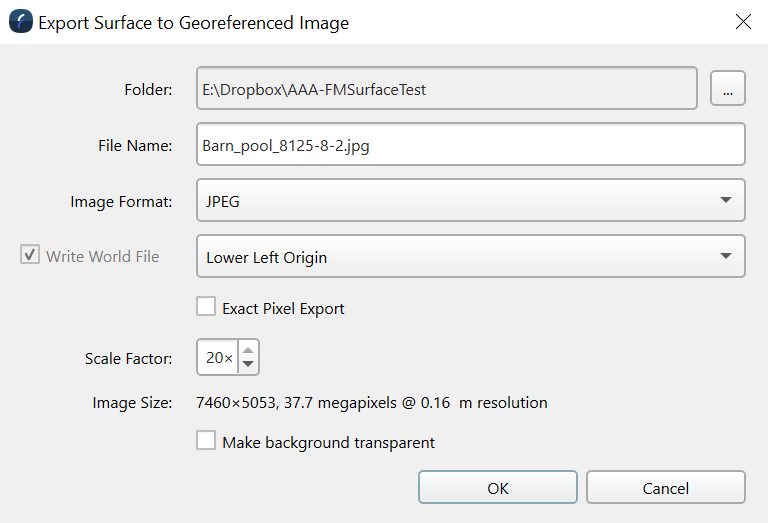
In particular you have a scale factor and the dialog will show you the resulting image size and effective resolution of each pixel in the image. Unlike the above method behind the scenes this method creates a canvas that exactly matches the aspect ration (width/height) of the surface with a resolution based on the scale factor. The rendering system then renders that surface with a top down orthographic projection into the resulting canvas and saves the results as a properly geo-referenced image. Given that the rendering system is used to generate the image it will appear identical (in colors and structure) to what you see in the 3D rendering of the surface. Generally the scale factor is adjust so the canvas is close to or slightly higher resolution then the surface being exported although if you have a high resolution texture on the surface you will want to select a resolution close to the draped textures resolution. The rendered project is considerably more flexible but it is import to understand the differences. There are two key issues.
Rendered pixel resolution vs surface cell size
Given the resulting rendered resolution generally differs from the exact cell size of the surface don't expect perfect pixel alignment with the exact pixel export. It will be within the size of the pixel resolution but unless you have a perfect match or integer multiple it won't be exact. However the resulting imagery will be where it is supposed to be
Differences based on rendering method
It is important to consider how we render surfaces for display in a 3D scene because the display engine makes some compromises for efficient high speed rendering. Also 3D rendering has some additional conditions that do not to be considered in more typical 2D GIS systems. In particular we make a compromise in how we handle data holes (data holidays/missing cells). It is this handling of missing data which often causes some confusion related to positioning when looking at visualized data. For a complete grid (no holes and a valid value for every cell) you will not see any apparent data shifts. The system renders shaded surfaces by joining cell centers together to create a rendered patch and the system will guarantee that if the lower left corner cell center has a value then the patch starting from that corner will be drawn. However, if the lower left cell centre is a data holiday then the corresponding patch will not be drawn. Thus the rendering of “holes” presents a challenge here because while a hole corresponds to the area of the empty bin the rendered hole is actually drawn from that cell centre to the next one to the upper right. This means that the hole will be visually shifted by half a cell although it will have the correct size (one cell area). While the small shift isn’t ideal it was considered the best compromise of various options considered. The advantage is that it allows the system to maintain maximize rendering efficiency, keeps the hole proper size, and makes sure that any point of the surface that has data will always be shown even if a single cell is surrounded by data holidays which is absolutely critical. This minor shift of the rendered hole position can be confusing if you are very carefully inspecting geo position at the hole's location.
The ability to render into a top down image is quite a useful feature and in particular it is used when rendering a scene to an image. If you have a complex scene with multiple surfaces, points, lines, or any other data you can always create a final properly geo-referenced image of all data together via the File > Export Scene To Image... option. The dialog box presented is similar to the surface to image export although the result is always a rendered product.
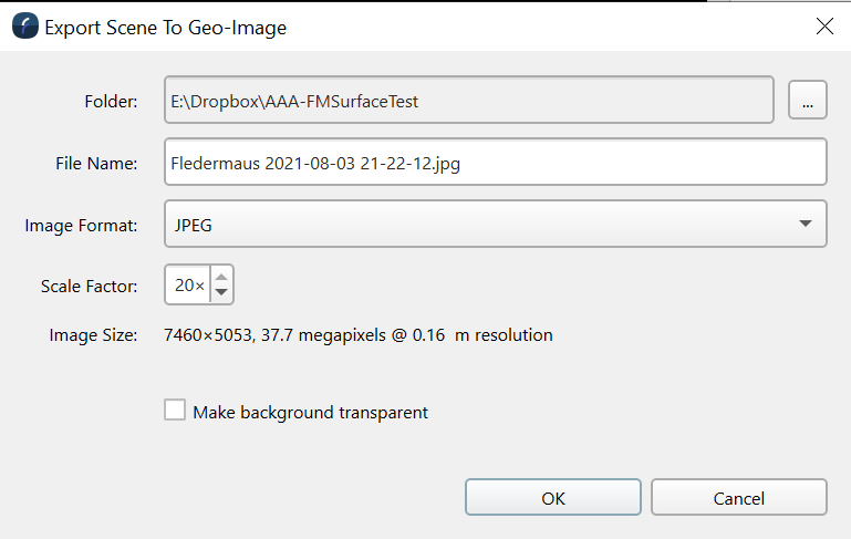
Currently the main limitation with the render to image process is it is limited to a maximum output resolution of 8192 x 8192 pixels although hopefully that limit will go away in a future release.